🌊 Tide

Information moves like the tide. We pick the waves worth studying.

中文

← Today's tide

Published 2026-07-16 · rednote-hilab · Xiangdong Zhang, Xiaohan Qin, Sunan Zou et al.

xHC: Expanded Hyper-Connections

arXiv · HuggingFace · ▲26

Abstract (verbatim)

Hyper-Connections (HC) expand the residual stream of Transformers into N parallel streams, providing a form of memory scaling beyond model width and depth. Manifold-Constrained HC (mHC) stabilizes this formulation at scale. The large gains from N{=}1 to N{=}4 suggest residual-stream expansion as a promising scaling axis. However, existing HC-family methods typically stop at N{=}4. Our experiments reveal why: scaling mHC beyond this point yields diminishing performance gains and rapidly increasing training cost. We attribute this limitation to two bottlenecks: insufficient write-back information for an expanding number of streams and residual-mixing generation whose cost scales cubically with N. To address both bottlenecks, we propose xHC (Expanded Hyper-Connections), the first HC-family method to achieve meaningful expansion beyond N{=}4. xHC combines temporal feature augmentation for richer write-back with a sparse residual-stream architecture that updates only k=4 of the N=16 streams while retaining dense access to the full residual state. Across 18B and 28B MoE models, xHC delivers strong and consistent downstream improvements. On an 18B MoE model, xHC improves the average downstream score by 4.0 points over mHC, while adding only modest training FLOPs over the vanilla baseline. Scaling-law experiments show that the vanilla and mHC require 1.50times and 1.19times the compute of xHC, respectively, to reach the same loss. Practical large-N training also requires controlling memory traffic from the expanded residual state. We therefore introduce xHC-Flash, which reduces the per-sublayer memory traffic from 73.5C to 40C, comparable to the 34C required by mHC at N{=}4, while retaining the gains of full xHC. Together, xHC and xHC-Flash make large-N residual-stream expansion effective and practical for LLM pre-training.

Background

Large language models (LLMs) have long relied on a single residual stream to pass information, a design that limits their ability to flexibly control cross-layer information. As models scale, simply increasing width, depth, or data volume no longer efficiently improves performance, creating a need for new scaling dimensions. Hyper-Connections (HC) technology attempts to add "memory capacity" to models through parallel residual streams and learnable mixing matrices, but existing methods hit bottlenecks when scaling beyond 4 parallel streams—performance gains diminish while computational costs surge.

Specifically, previous approaches face two key flaws: first, each new residual stream needs to store different layer output histories, but each layer can only inject a single write-back signal, leading to insufficient information diversity; second, computational costs grow cubically with the number of streams because they need to predict mixing coefficients from high-dimensional states. This makes scaling residual streams "expensive and inefficient."

The proposed xHC (Expanded Hyper-Connections) solves these problems with a two-pronged approach: it introduces temporal feature augmentation to provide richer context information for each residual stream while maintaining computational efficiency, and adopts a sparse residual stream architecture that only activates a few streams for updates, significantly reducing computational overhead. This design addresses both information diversity and computational cost issues, making residual stream expansion to 16 or more streams feasible.

Compared to previous work, xHC's key innovations include: 1) achieving effective expansion beyond 4 parallel streams for the first time; 2) decoupling but synergistically combining information enhancement with computational optimization; 3) not only improving performance but also significantly enhancing the cost-effectiveness of scaling. Experiments show that on an 18B-parameter MoE model, xHC improves downstream task scores by 4 points over the existing method mHC while adding only minimal training costs. This breakthrough makes residual stream expansion a truly effective scaling dimension for LLM training.
Method, Figure by Figure

M E T H O D1 / 7

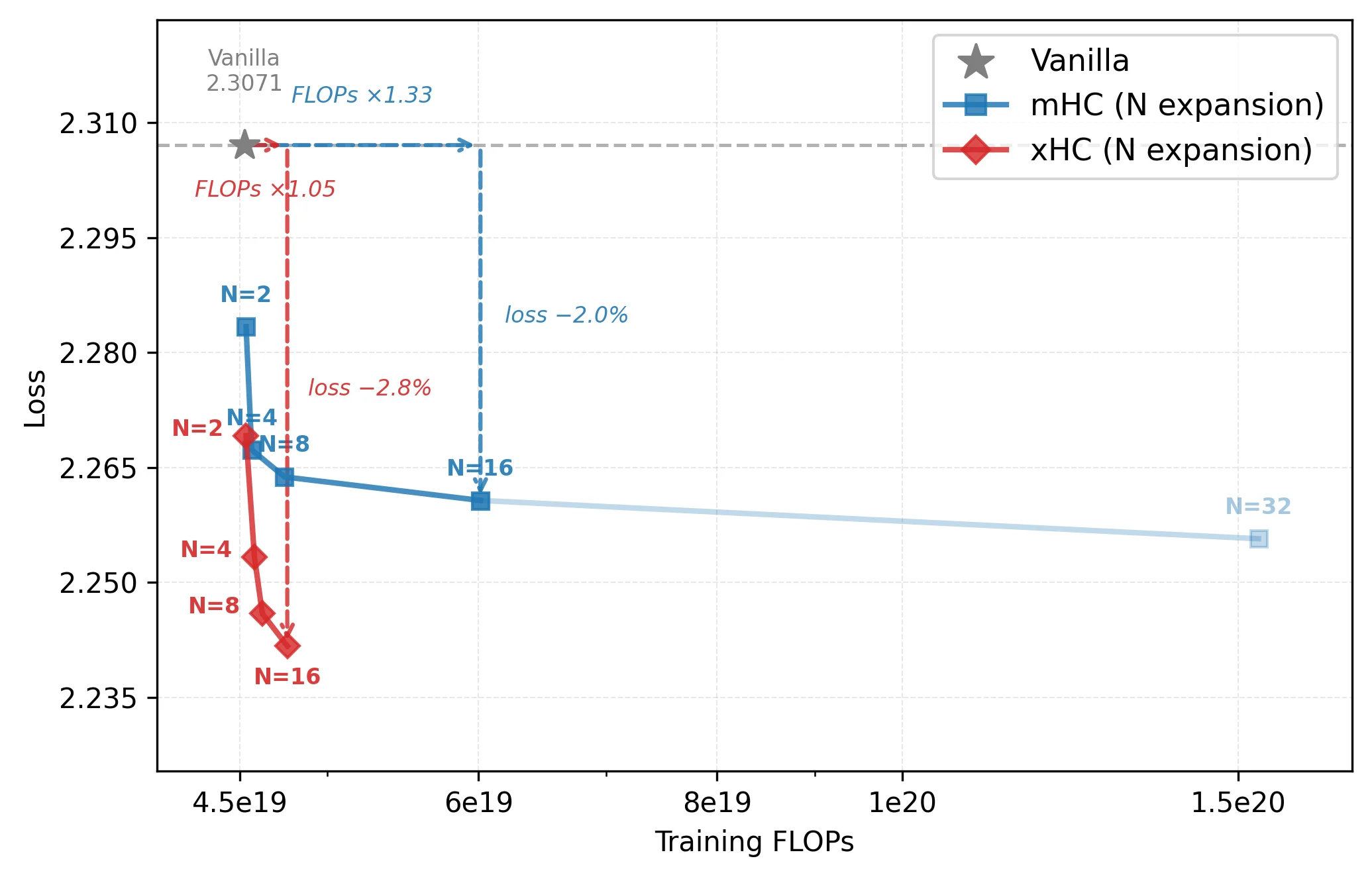
Figure 1 : Expansion efficiency: loss vs. FLOPs on a 2.5B MoE model (details in Table 6 ).

This figure (Figure 1) illustrates the relationship between "Loss" and "Training FLOPs" for different methods on a 2.5B MoE model, comparing their scaling efficiency. The horizontal axis represents "Training FLOPs," indicating the computational cost required during training, with values increasing from left to right. The vertical axis represents "Loss," indicating the model's loss value, with values decreasing from top to bottom, meaning better model performance.

Three methods are compared in the graph: Vanilla (marked with gray stars), mHC (N expansion) (marked with blue squares), and xHC (N expansion) (marked with red diamonds). Each method has experimental points for different N values, where N represents the number of parallel streams for scaling.

1. Vanilla Method:

  • It has only one data point (gray star) located in the top-left corner of the graph, corresponding to approximately 4.5e19 FLOPs and a Loss of about 2.3071. This represents the baseline model without any HC scaling. A horizontal dashed line extends from this point to the right, labeled "FLOPs ×1.33," pointing to the FLOPs position of mHC at N=16. This indicates that to achieve similar performance (Loss of about 2.265) as mHC (N=16), the Vanilla method would need to increase its computational cost by approximately 33%.

2. mHC (N expansion) Method:

  • This is a blue curve showing the changes in Loss and FLOPs as N (2, 4, 8, 16, 32) increases.
  • When N increases from 2 to 4, FLOPs change slightly, but Loss decreases significantly (from about 2.280 to about 2.265).
  • When N increases from 4 to 8, Loss continues to decrease, but the rate of decrease slows down.
  • When N increases from 8 to 16, Loss further decreases, but the curve starts to flatten. From N=16 to N=32, FLOPs increase significantly (from about 6e19 to about 1.5e20), but the decrease in Loss is very limited (from about 2.265 to just below 2.260). The blue dashed arrow from N=16 to N=32 is labeled "loss −2.0%," indicating a very small reduction in loss.
  • This suggests that mHC is effective in reducing loss when N is small (e.g., N=4 or 8), but as N increases further (e.g., N>16), the increase in computational cost far outpaces the performance improvement, leading to diminishing returns.

3. xHC (N expansion) Method:

  • This is a red curve showing the changes in Loss and FLOPs as N (2, 4, 8, 16) increases.
  • When N increases from 2 to 4, FLOPs increase slightly (from about 4.5e19 to just above 4.5e19), but Loss decreases significantly (from about 2.280 to about 2.265).
  • When N increases from 4 to 8, Loss continues to decrease, and FLOPs also increase.
  • When N increases from 8 to 16, Loss decreases significantly further (from about 2.265 to about 2.240), while the increase in FLOPs is relatively small (from just above 4.5e19 to about 5.5e19).
  • The red dashed arrow from the Vanilla method to xHC (N=16) is labeled "FLOPs ×1.05," indicating that xHC (N=16) achieves a lower loss with only about 5% more computational cost than the Vanilla method.
  • The red dashed arrow from xHC (N=4) to xHC (N=16) is labeled "loss −2.8%," indicating a significant reduction in loss within this range of N.

Revealing the Mechanism of Operation:

  • mHC: Scales residual streams by increasing the number of parallel streams N. However, as shown in the figure, it exhibits diminishing returns when N exceeds a certain value (e.g., 16) because the computational cost (FLOPs) increases rapidly while performance improvement is limited. This may be due to bottlenecks such as "insufficient write-back information" and "residual mixing generation cost increasing cubically with N."
  • xHC: Aims to address the bottlenecks encountered by mHC at large N values. It achieves this through two methods: 1) "Temporal Feature Enhancement" to provide richer write-back information; 2) "Sparse Residual Stream Architecture," where only k=4 out of N streams are updated while maintaining dense access to the entire residual state. This allows xHC to effectively reduce loss even at large N values (e.g., N=16) while controlling the increase in computational cost.

Conclusion:

  • The figure clearly demonstrates the superiority of the xHC method over mHC and Vanilla.
  • Efficiency Comparison: xHC achieves lower loss with a smaller increase in computational cost. For example, xHC (N=16) achieves a significant reduction in loss with only about 5% more computational cost than Vanilla. In contrast, mHC requires a larger increase in computational cost to achieve similar performance improvements or shows limited performance improvement with the same computational cost.
  • Scalability: xHC proves that scaling residual streams (N>4) is a promising direction, while mHC is inefficient at large N values. xHC addresses the bottlenecks of large N scaling with its innovative architecture, achieving meaningful performance improvements.
  • Key Findings: At N=16, xHC requires only about 5% additional FLOPs compared to Vanilla to achieve better performance; at N=16, mHC's FLOPs are approximately 1.33 times those of Vanilla (inferred from the horizontal dashed line). The xHC curve at N=16 is significantly lower than the mHC curve, indicating better performance at the same or lower computational cost.

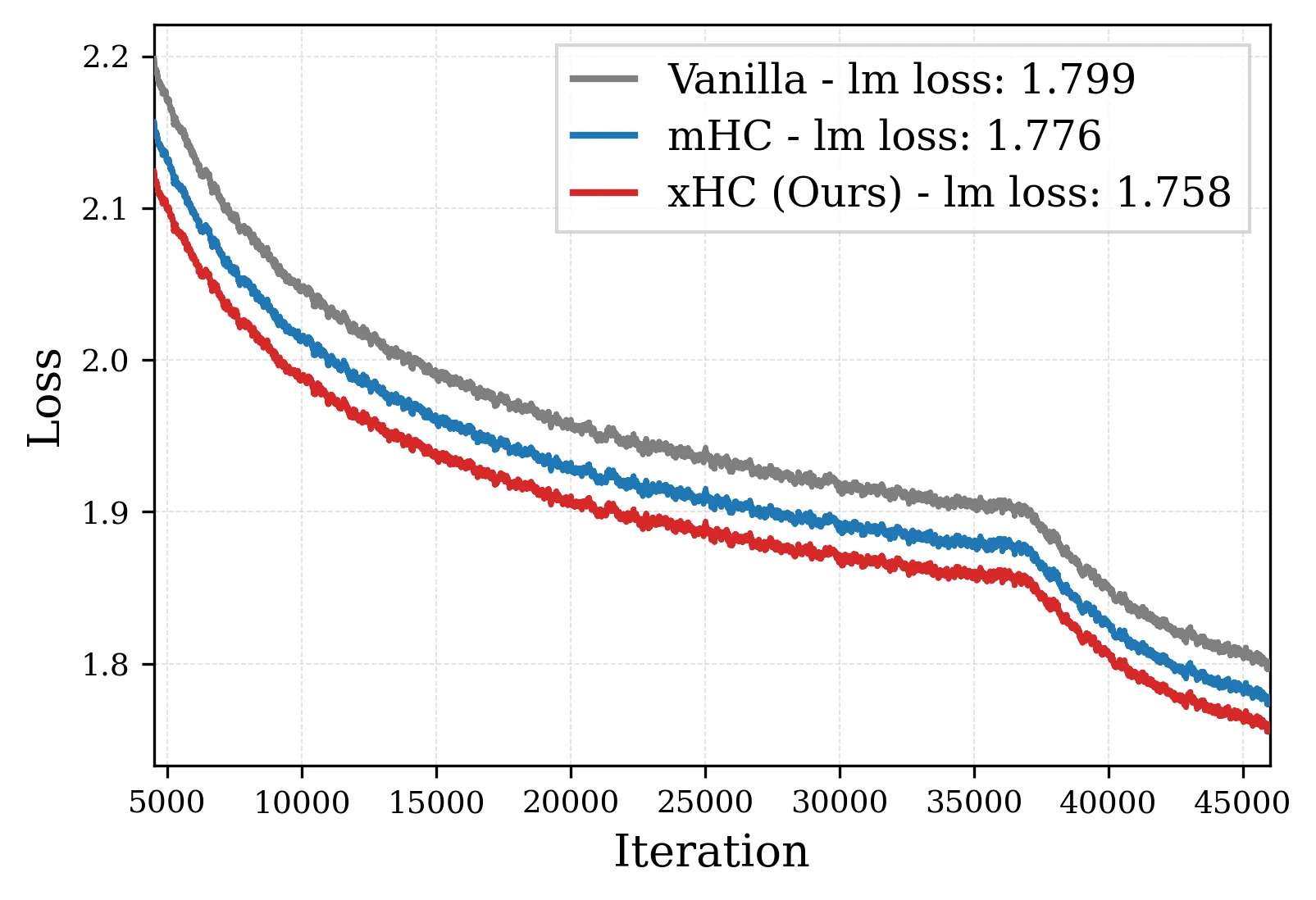
(a) Training loss. (b) Average downstream score. (c) Benchmark-level gains. Figure 2 : xHC delivers broad gains at 18B scale. (a) xHC achieves lowest training loss. (b) The loss improvement translates into a significantly higher average downstream score across benchmarks in Table 1 . (c) xHC improves representative benchmarks across reasoning, knowledge, and code.

This figure (Figure 2a) displays the curves of loss over iterations for three different methods during the training process, used to compare their training effectiveness.

Explanation of Components in the Figure

  • Horizontal Axis (Iteration): Represents the number of training iterations, ranging from 5000 to 45000, indicating how many times the model has been updated during training. A larger number means the training has been going on for a longer time.
  • Vertical Axis (Loss): Represents the training loss. A lower value indicates a better training effect of the model (i.e., the model fits the task better).
  • Three Curves:
  • Gray Curve (Vanilla): Represents the training loss of the original model (without using HC - related improvements). Its final average language model loss (lm loss) is 1.799.
  • Blue Curve (mHC): Represents the training loss of the model using the Manifold - Constrained Hyper - Connections (mHC) method. The final average language model loss is 1.776.
  • Red Curve (xHC (Ours)): Represents the training loss of the model using the xHC (Expanded Hyper - Connections) method proposed in this paper. The final average language model loss is 1.758.

Operating Principle of the Methods (Inferred from the Figure Results)

  • From the downward trend of the loss curves, the losses of the three methods decrease as the number of iterations increases, indicating that they can all improve the model performance through training.
  • The curve of xHC (red) is below the curves of mHC (blue) and Vanilla (gray) for most of the iteration counts, which shows that xHC can more effectively reduce the loss during training. Combining with the content of the paper, xHC provides richer write - back information through temporal feature augmentation, solving the problem of insufficient write - back information of mHC when the number of parallel streams (N) is large; at the same time, it adopts a sparse residual - stream architecture, updating only k = 4 out of N = 16 streams while maintaining dense access to the complete residual state, solving the problem that the cost of residual mixing generation grows cubically with N. Thus, it can achieve meaningful scaling at a larger N and obtain a better loss reduction effect during training.

Coordinates, Comparison Objects, and Conclusion

  • Coordinates: The horizontal axis is the number of iterations (from 5000 to 45000), and the vertical axis is the loss (around 1.8 to 2.2).
  • Comparison Objects: Vanilla (original model), mHC (existing improved method), xHC (method proposed in this paper).
  • Conclusion: Among these three methods, xHC has the lowest training loss (the final lm loss is 1.758), and in the entire training process (from iteration 5000 to 45000), both the speed of loss reduction and the final loss value are better than those of mHC and Vanilla. This shows that xHC can optimize the model more effectively during the training stage, laying a foundation for achieving better results in subsequent downstream tasks (such as reasoning, knowledge, and code - related benchmark tests) (combining with the content of downstream scores and benchmark test gains in the subsequent part of the paper, it can be inferred that a low training loss helps to improve downstream performance). At the same time, from the perspective of training computational efficiency (mentioned in the paper), vanilla and mHC need 1.50 times and 1.19 times more computational resources than xHC to achieve the same loss, which also shows that xHC has advantages in both training efficiency and performance.

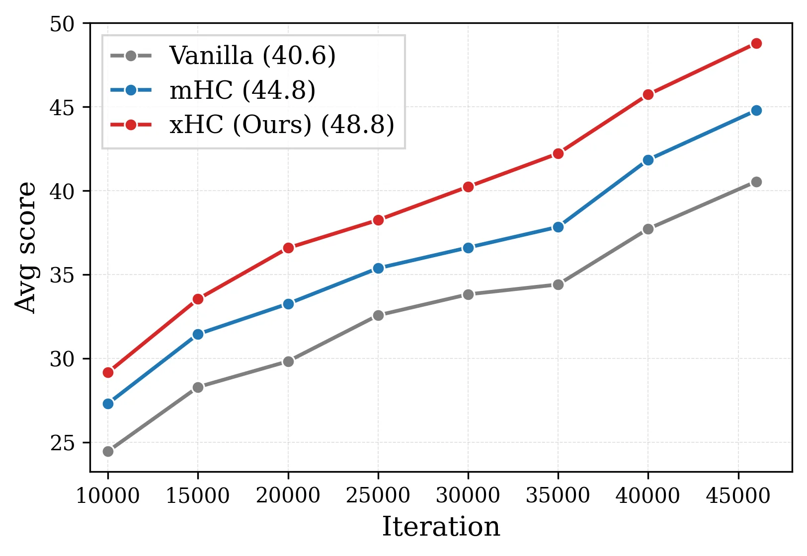
(a) Training loss. (b) Average downstream score. (c) Benchmark-level gains. Figure 2 : xHC delivers broad gains at 18B scale. (a) xHC achieves lowest training loss. (b) The loss improvement translates into a significantly higher average downstream score across benchmarks in Table 1 . (c) xHC improves representative benchmarks across reasoning, knowledge, and code.

This figure (Figure 2b) illustrates the trend of the average downstream score for three different methods as a function of iteration count during training, clearly comparing their performance and rate of improvement.

First, let's break down the components of the graph: - X-axis (Horizontal Axis): Represents the "Iteration" of training, ranging from 10,000 to 45,000. This indicates the progress of model training, with larger numbers signifying more advanced training stages. - Y-axis (Vertical Axis): Represents the "Avg score," ranging approximately from 25 to 50. This score is an aggregate performance of the model across a series of downstream benchmark tests, where a higher score indicates better model performance. - Three Curves: Each curve represents a different method: - Gray Curve (Vanilla): This typically refers to a baseline Transformer model without the specific HC (Hyper-Connections) method. The legend indicates an average score of 40.6 (possibly at a specific iteration or final average score). - Blue Curve (mHC): Represents the "Manifold-Constrained HC" method. The legend indicates an average score of 44.8. - Red Curve (xHC (Ours)): Represents the "Expanded Hyper-Connections" method proposed in the paper, i.e., the authors' method. The legend indicates an average score of 48.8.

The flow of data and presentation of information are as follows: - Each point on the curves represents the average downstream score of the corresponding method at a specific iteration count. - As the iteration count increases (from left to right), the scores for all methods show an upward trend, indicating that the model's performance improves with more training. - We can observe the rate of improvement and the final score levels for different methods: - Vanilla Method (gray curve): The score increases relatively slowly, with a final average score of 40.6. - mHC Method (blue curve): The score increases faster than Vanilla, with a final average score of 44.8. - xHC Method (red curve): The score increases the fastest, with a final average score of 48.8, significantly higher than the other two methods.

This figure reveals how the method works and its effectiveness: - Advantages of xHC: By combining "temporal feature augmentation" to provide richer write-back information and a "sparse residual-stream architecture" (updating only k=4 out of N=16 streams while retaining dense access to the full residual state), xHC achieves meaningful expansion at larger N values. This enables xHC to use resources more effectively and achieve better performance on downstream tasks during training. - Performance Comparison: From the graph, it is clear that xHC outperforms both mHC and Vanilla methods at all iteration stages. Especially in the later stages of training, xHC shows a more significant increase in score, ultimately achieving the highest average downstream score. This indicates that xHC not only improves model performance but also accelerates the convergence process. - Computational Efficiency: Although the graph does not directly show computational cost, according to the paper's abstract, xHC requires less computational effort (FLOPs) to reach the same loss compared to Vanilla and mHC. This means that xHC can achieve performance improvements while maintaining lower computational costs.

Conclusion: This figure clearly demonstrates that the xHC method proposed in the paper achieves significant downstream performance improvements in 18B-scale MoE models. Compared to mHC and Vanilla methods, xHC can more quickly increase the average downstream score during training and ultimately reach a higher score level. This verifies the effectiveness of the xHC method in addressing the bottlenecks encountered by HC-family methods at large N values and showcases its potential in practical applications.

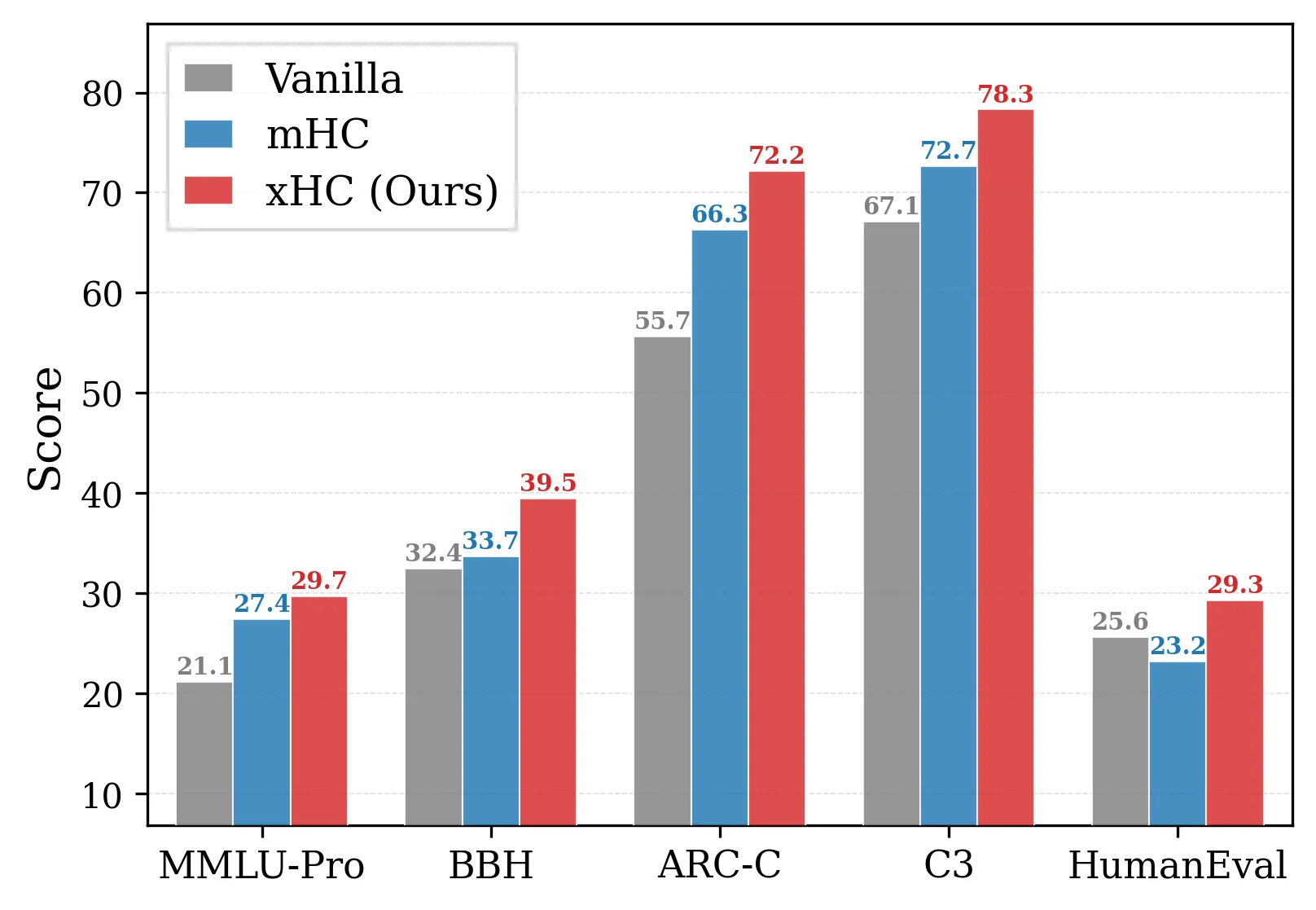
(a) Training loss. (b) Average downstream score. (c) Benchmark-level gains. Figure 2 : xHC delivers broad gains at 18B scale. (a) xHC achieves lowest training loss. (b) The loss improvement translates into a significantly higher average downstream score across benchmarks in Table 1 . (c) xHC improves representative benchmarks across reasoning, knowledge, and code.

This figure (part (c) of Figure 2, labeled "Benchmark-level gains") illustrates the performance scores of different methods across multiple benchmark tests, demonstrating that xHC (our method) outperforms Vanilla (baseline method) and mHC (existing method) on these benchmarks. Let’s first examine the axes: the vertical axis represents "Score" (ranging from 10 to 80), while the horizontal axis lists the benchmark tests, including MMLU-Pro, BBH, ARC-C, C3, and HumanEval.

Each benchmark has three bars representing the three methods:
- The gray bar corresponds to the Vanilla method (baseline).
- The blue bar represents the mHC method.
- The red bar denotes our xHC method (labeled "Ours").

Analysis of Each Benchmark:

  1. MMLU-Pro:
  2. Vanilla: 21.1
  3. mHC: 27.4
  4. xHC: 29.7
    xHC outperforms mHC, which in turn outperforms Vanilla, indicating better performance on this knowledge-based benchmark.

  5. BBH:

  6. Vanilla: 32.4
  7. mHC: 33.7
  8. xHC: 39.5
    xHC achieves a significantly higher score than both mHC and Vanilla, showing a notable improvement.

  9. ARC-C:

  10. Vanilla: 55.7
  11. mHC: 66.3
  12. xHC: 72.2
    xHC’s score is substantially higher than the other two, highlighting its stronger performance on reasoning-based benchmarks.

  13. C3:

  14. Vanilla: 67.1
  15. mHC: 72.7
  16. xHC: 78.3
    xHC achieves the highest score, with an even wider gap compared to the other methods, demonstrating its effectiveness on large-scale reasoning or knowledge benchmarks.

  17. HumanEval (a code-related benchmark):

  18. Vanilla: 25.6
  19. mHC: 23.2 (mHC scores slightly lower than Vanilla here, possibly due to task-specific adaptability).
  20. xHC: 29.3
    xHC significantly outperforms both, indicating strong performance in code generation tasks.

Overall Trend:

xHC achieves higher scores than both Vanilla and mHC across all benchmarks (except for HumanEval, where mHC scores slightly below Vanilla, but xHC still far exceeds both). This demonstrates that xHC effectively enhances model performance on downstream benchmarks, regardless of whether they involve knowledge, reasoning, or code generation.

In the context of the paper, xHC addresses the bottleneck issues of mHC in large-scale settings (N > 4) by incorporating time-feature enhancement (richer write-back) and a sparse residual flow architecture (updating only k=4 out of N=16 flows while maintaining dense access to the full residual state). The results in this figure validate xHC’s effectiveness, showing broad performance improvements across multiple benchmarks—particularly for 18B-scale models, where it achieves an average downstream score 4.0 points higher than mHC, with a relatively moderate increase in training FLOPs.

Conclusion:

By comparing the three methods (Vanilla, mHC, and xHC) across five benchmarks, this figure clearly highlights xHC’s advantages: it achieves higher scores across all benchmarks, proving its ability to enhance model performance on downstream tasks. It also resolves the issues of diminishing performance gains and increased training costs associated with scaling large N in existing HC-family methods.

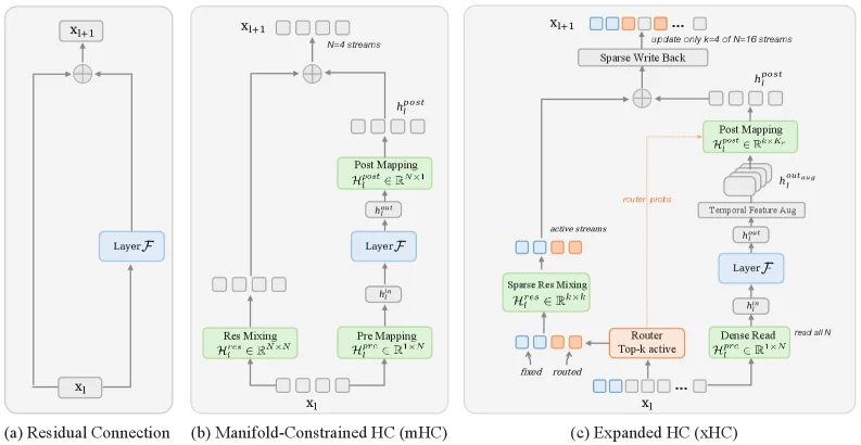
Figure 3 : Overview of xHC. (a) A standard Transformer layer maintains a single residual stream. (b) mHC expands the residual state into N = 4 N{=}4 streams with dense residual mixing and write-back. (c) xHC scales to N = 16 N{=}16 with only k = 4 k{=}4 active streams: it reads all streams, applies the sublayer ℱ \mathcal{F} (Attn/MLP), augments MLP outputs, and sparsely writes back to selected streams. Blue/orange streams denote fixed/routed active streams. Restricting residual mapping to the k k active streams reduces the dominant residual-mapping generation cost from O ​ ( N 3 ​ C ) O(N^{3}C) to O ​ ( k 3 ​ C ) O(k^{3}C) .

This figure (Figure 3) illustrates the evolution from standard Transformer residual connections to mHC (Manifold-Constrained HC) and then to xHC (Expanded Hyper-Connections), helping us understand the working mechanism of xHC:

Subfigure (a): Residual Connection in a Standard Transformer Layer

  • Components and Flow: There is only one residual flow here. The input is \( x_1 \). After being processed by the blue "Layer \( \mathcal{F} \)" (which can be an attention or MLP sublayer), it is combined with the original input \( x_1 \) through an addition operation (\( \oplus \)) to obtain the output \( x_{t + 1} \). The data flow order is \( x_1 \rightarrow \text{Layer } \mathcal{F} \rightarrow \oplus \text{ (adding with } x_1 \text{)} \rightarrow x_{t + 1} \). This represents the computational process of a single residual flow in traditional Transformers, where all computations are performed on this single flow.

Subfigure (b): mHC (Manifold-Constrained HC)

  • Components and Flow: mHC expands the residual state to \( N = 4 \) flows.
    • First, the input \( x_1 \) enters the "Pre Mapping \( \mathcal{H}_{\text{pre}}^{\text{res}} \in \mathbb{R}^{1 \times N} \)" (pre-mapping, which maps the input to the space of \( N \) flows), and then it is divided into \( N = 4 \) flows (represented by multiple small squares in the figure).
    • One of the flows is processed by "Layer \( \mathcal{F} \)" to obtain \( h^u \). Then \( h^u \) enters the "Post Mapping \( \mathcal{H}{\text{post}}^{\text{res}} \in \mathbb{R}^{N \times 1} \)" (post-mapping, which maps the space of \( N \) flows back to a single space), and then combines with the previous \( N \) flows through "Res Mixing \( \mathcal{H}{\text{res}}^{\text{res}} \in \mathbb{R}^{N \times N} \)" (residual mixing, which mixes the information of \( N \) flows) and an addition operation (\( \oplus \)). Finally, \( x_{t + 1} \) is obtained. In addition, there are \( N = 4 \) flows that directly combine with the previous result through an addition operation (\( \oplus \))? No, let's re-examine: the input \( x_1 \) goes through Pre Mapping to get \( N \) flows. One of the flows goes through Layer \( \mathcal{F} \) to \( h^u \), and \( h^u \) goes to Post Mapping. Then the output of Post Mapping and \( N \) flows (including the original \( N \) flows? Or the \( N \) flows after Pre Mapping?) are mixed through Res Mixing. Then it is added with \( N = 4 \) flows (possibly part of the \( N \) flows after Pre Mapping?) to get \( x_{t + 1} \)? In fact, the core is that mHC expands the residual flow to \( N = 4 \), using dense residual mixing (Res Mixing, with a complexity of \( O(N^3C) \)) and dense write-back (all \( N \) flows participate in write-back). This can utilize the information of multiple flows, but it also brings the problem of computational cost, especially when \( N \) increases.

Subfigure (c): xHC (Expanded Hyper-Connections)

  • Components and Flow: xHC expands to \( N = 16 \) flows, but only \( k = 4 \) flows are active (updated).
    • Read (Dense Read): First, the input \( x_1 \) (or the current residual state) is read by "Dense Read", that is, all \( N = 16 \) flows are read (the figure shows "read all \( N \)"), to obtain \( \mathcal{H}_{\text{pre}}^{\text{res}} \in \mathbb{R}^{1 \times N} \).
    • Sublayer Processing (Layer \( \mathcal{F} \)): Then, these \( N = 16 \) flows are processed by "Layer \( \mathcal{F} \)" (attention or MLP sublayer) to obtain \( h^u \) (possibly an intermediate result).
    • Temporal Feature Aggregation (Temporal Feature Agg): For the active flows (blue/orange in the figure, blue is fixed, orange is routed), their MLP outputs (\( h_{\text{temp}}^{\text{fixed}} \) and \( h_{\text{temp}}^{\text{routed}} \)? Or the processing after MLP output) will go through "Temporal Feature Agg" (temporal feature aggregation). This step is to generate richer write-back information to solve the problem of insufficient write-back information in mHC.
    • Sparse Residual Mixing (Sparse Res Mixing): Then, "Sparse Res Mixing \( \mathcal{H}_{\text{res}}^{\text{res}} \in \mathbb{R}^{k \times k} \)" (because only \( k = 4 \) flows are active, the complexity is reduced from \( O(N^3C) \) to \( O(k^3C) \)) is performed. Here \( k = 4 \), so the information of these \( k \) active flows is mixed.
    • Routing (Router Top - k - active): The "Router" selects \( k = 4 \) active flows (the orange "routed" flows and blue "fixed" flows in the figure? Or selects \( k = 4 \) active flows from \( N = 16 \) flows) to determine which flows will be updated.
    • Sparse Write Back (Sparse Write Back): Finally, "Sparse Write Back" only updates \( k = 4 \) active flows (the figure shows "update only \( k = 4 \) of \( N = 16 \) streams"), while the other \( N - k = 12 \) flows remain unchanged (or use previous information?). The data flow order is: \( x_1 \rightarrow \text{Dense Read (all } N \text{ streams)} \rightarrow \text{Layer } \mathcal{F} \rightarrow \text{(temporal feature aggregation of active flows)} \rightarrow \text{Sparse Res Mixing (} k = 4 \text{ streams)} \rightarrow \text{Router (select } k = 4 \text{ active streams)} \rightarrow \text{Sparse Write Back (update } k = 4 \text{ streams)} \rightarrow x_{t + 1} \) (at the same time, the non-active flows may be directly transmitted? Or combined with the write-back flows? There is also an addition operation \( \oplus \) in the figure, which may be to add the write-back \( k \) flows with the other \( N - k \) flows?).

Core Operating Mode of the Method

  • Expand the Number of Flows: xHC expands the residual flow from \( N = 4 \) in mHC to \( N = 16 \), but reduces the computational cost through sparse update (only updating \( k = 4 \) flows).
  • Solve the Bottleneck of mHC:
    • Insufficient Write-Back Information: Through "Temporal Feature Agg" to perform temporal feature aggregation on the MLP output, richer write-back information is generated, so that the updated \( k \) flows can obtain sufficient information.
    • High Cost of Residual Mixing: By performing "Sparse Res Mixing" only on \( k = 4 \) active flows, the complexity of residual mixing is reduced from \( O(N^3C) \) (when \( N = 4 \) in mHC, it is \( O(4^3C) \); when \( N = 16 \) but \( k = 4 \) in xHC, it is \( O(4^3C) \)) to solve the problem of cubic growth of residual mixing cost when \( N \) increases in mHC.
  • Key Steps of Data Flow: Read the information of all flows, after sublayer processing, enhance the output of active flows, sparsely mix these active flows, and then only update these \( k \) active flows. The non-active flows are retained or use previous information (combined through an addition operation?).

Comparison with mHC (Inferred from the Figure)

  • Number of Flows: mHC is \( N = 4 \), xHC is \( N = 16 \), but xHC only updates \( k = 4 \) flows.
  • Computational Cost: The complexity of residual mixing in mHC is \( O(N^3C) \) (when \( N = 4 \), it is \( O(64C) \)), and that in xHC is \( O(k^3C) \) (when \( k = 4 \), it is \( O(64C) \), but if mHC is used when \( N = 16 \), the complexity is \( O(4096C) \)). So the computational cost of xHC grows slowly when \( N \) increases.
  • Write-Back Information: mHC is dense write-back (all \( N \) flows participate), but the write-back information may be insufficient; xHC provides richer write-back information through temporal feature aggregation, and only updates \( k \) flows at the same time, solving the problems of insufficient write-back information and high computational cost.

This figure clearly shows how xHC solves the bottleneck of mHC by expanding the number of residual flows while using sparse update and temporal feature enhancement, so as to achieve meaningful expansion (beyond \( N = 4 \)).

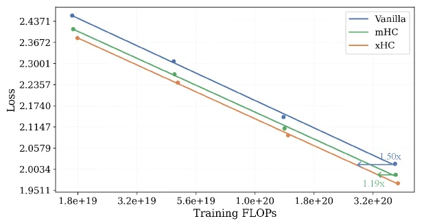
Figure 4 : Scaling-law comparison. xHC traces a consistently lower loss curve than both mHC and the vanilla residual baseline across training compute.

This figure (Figure 4) presents a scaling - law comparison among different methods in terms of the relationship between training computational cost (measured by training FLOPs) and loss. The horizontal axis is "Training FLOPs" (number of floating - point operations during training). As we move from left to right, the value increases, which means more computational resources are invested in the training process. The vertical axis is "Loss". As the value decreases from top to bottom, it indicates that the model's performance is getting better (a lower loss usually means a better prediction or learning effect of the model).

There are three curves in the figure, each representing a different method: - The blue curve (Vanilla): It represents the Transformer model with basic residual connections (vanilla residual), serving as the baseline method. - The green curve (mHC): It stands for Manifold - Constrained Hyper - Connections (mHC). This method is used to stabilize the hyper - connection formula at a large scale. - The orange curve (xHC): It represents Expanded Hyper - Connections (xHC), a new method proposed in the paper. Its purpose is to solve the problems of decreasing performance gains and rapidly increasing training costs when mHC is scaled to a large N (the number of hyper - connection streams).

As we can see from the figure, as the training FLOPs increase, the loss of all three methods decreases, which conforms to the general law of model training: more computational resources usually lead to better model performance (lower loss). However, the key is that the rate of loss reduction and the final loss level are different for different methods.

Specifically, under the same training FLOPs, the loss curve of xHC is always lower than those of mHC and Vanilla. For example, on the right side of the figure, when the training FLOPs reach 3.2e + 20, the loss of xHC is lower than that of mHC, and the loss of mHC is lower than that of Vanilla. The figure also marks the computational efficiency of xHC relative to mHC and Vanilla: When xHC achieves the same loss as mHC, the required training FLOPs are only 1/1.19 of those of mHC (that is, the computational cost required by mHC is 1.19 times that of xHC); when xHC achieves the same loss as Vanilla, the required training FLOPs are only 1/1.50 of those of Vanilla (that is, the computational cost required by Vanilla is 1.50 times that of xHC). This shows that xHC has a higher training efficiency, as it can achieve a lower loss with the same training computational cost, or it requires less training computational cost to achieve the same loss.

From the perspective of how the method works, xHC combines temporal feature augmentation to provide richer write - back information, solving the problem of insufficient write - back information when the number of hyper - connection streams is expanded. At the same time, it adopts a sparse residual - stream architecture, which only updates k = 4 out of N = 16 streams while retaining dense access to the full residual state, solving the problem that the cost of residual - mixing generation grows cubically with N. In this way, xHC can achieve meaningful expansion at a larger N, thus achieving a better balance between training computational cost and model performance. Compared with mHC and Vanilla methods, xHC can achieve a lower loss under the same training computational cost, or obtain a better model performance improvement with the same training computational cost.

To sum up the results of this figure: xHC performs better than mHC and the Vanilla residual baseline in the training scaling law. That is, under the same training computational cost, the loss of xHC is lower; or to achieve the same loss, the training computational cost required by xHC is less than that of mHC and Vanilla. This shows that xHC is a more efficient training method, which can provide better model performance without significantly increasing the training cost, or achieve better model performance improvement with the same training cost.

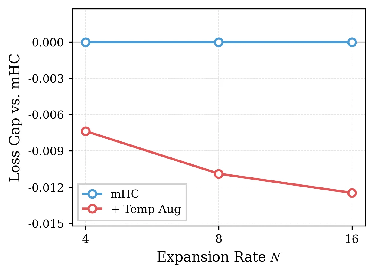
Table 2 : Ablation study. Parentheses show extra training FLOPs over vanilla baseline. “Sparse” is the sparse architecture, “D. Read” is Dense Read, and “Fixed” is the number of always-active streams. Figure 5 : Information bottleneck ablation. The gain grows with N N .

This figure is a result graph of the "Information Bottleneck Ablation Experiment" from the paper "xHC: Expanded Hyper-Connections," used to show the loss gap between different methods at various expansion rates.

Interpretation of Components and Information in the Graph

  1. X-axis: Labeled "Expansion Rate N," it represents the expansion rate of Hyper-Connections (HC), i.e., the number of parallel streams. The graph shows three expansion rates: 4, 8, and 16. This means the system is configured with 4, 8, or 16 parallel residual streams.

  2. Y-axis: Labeled "Loss Gap vs. mHC," it represents the loss gap relative to the "Manifold-Constrained HC (mHC)" method. The loss values are negative, meaning these methods have lower loss than mHC. The smaller the value (i.e., the more negative), the better the performance relative to mHC (lower loss).

  3. Curves and Data Points:

    • Blue Curve (with hollow circles): Represents the "mHC" method. This line is almost horizontal and has a value of 0.000 on the Y-axis. This indicates that the mHC method is used as a baseline, and its loss gap is defined as 0. The loss gaps of other methods are measured relative to this baseline.
    • Red Curve (with hollow circles): Represents the "+ Temp Aug" method, i.e., the method with "Temporal Feature Augmentation" applied. This curve shows a downward trend from left to right (the value becomes more negative). Specifically:
      • When the expansion rate N=4, the loss gap is approximately -0.010 (better than mHC).
      • When N=8, the loss gap is approximately -0.011 (better than N=4).
      • When N=16, the loss gap is approximately -0.012 (better than N=8).

How the Method Works (Inferred from the Graph)

This graph reveals how the "+ Temp Aug" method improves performance by increasing the expansion rate (N): * Temporal Feature Augmentation: This method provides richer "write-back" information to the system by introducing temporal feature augmentation. This enables the system to better handle the increased number of parallel streams as the expansion rate increases. * Improvement in Loss Gap: As the expansion rate N increases from 4 to 16, the loss of the "+ Temp Aug" method continuously decreases (becomes more negative), indicating that its performance relative to the mHC baseline is constantly improving. This suggests that temporal feature augmentation helps alleviate the diminishing performance gains of mHC when scaled to larger N.

Conclusion

  • Performance Comparison: At all shown expansion rates (N=4, 8, 16), the loss of the "+ Temp Aug" method is lower than the mHC baseline.
  • Scalability: The "+ Temp Aug" method shows good scalability, meaning that as the expansion rate N increases, its performance advantage (loss gap) over mHC also increases.
  • Alleviation of Information Bottleneck: This graph supports the paper's view that temporal feature augmentation can alleviate the information bottleneck problem of HC methods when scaling, thus still achieving performance improvements at larger expansion rates.

In summary, this graph clearly shows how the "+ Temp Aug" method improves performance by increasing the expansion rate. Relative to the mHC baseline, its loss continuously decreases, indicating that this method is more effective in handling large-scale hyper-connections.

← → flip · ↑ ↓ scroll notes · Esc exit