🌊 Tide

Information moves like the tide. We pick the waves worth studying.

中文

← Today's tide

Published 2026-07-16 · National University of Singapore, The Hong Kong Polytechnic University · Qi Li, Xingyi Yang, Xinchao Wang

BadWAM: When World-Action Models Dream Right but Act Wrong

arXiv · HuggingFace · ▲47

Abstract (verbatim)

World-action models (WAMs) are emerging as a promising foundation for embodied control: rather than predicting actions alone, they learn representations that couple action generation with future world prediction. This coupling is often viewed as a source of robustness, interpretability, and safety, as a robot's action can in principle be checked against its imagined future. In this paper, we show that this assumption is fragile. We introduce BadWAM, a unified framework for modeling and evaluating World-Action Drift Attacks: a new class of WAM-specific adversarial attacks that use small visual perturbations to break the alignment between what a WAM imagines and what it executes. BadWAM characterizes this attack surface along two natural criteria: attack strength and stealthiness. When the adversary prioritizes disruption, BadWAM instantiates an action-only adversarial attack, which directly drives the model toward task-failing actions. When the adversary additionally prioritizes stealth, BadWAM instantiates an imagination-preserving adversarial attack, which seeks to induce harmful action shifts while keeping the model's predicted future close to its clean imagination. Together, these two attacks capture a spectrum of WAM-specific failures: from overt action hijacking to stealthier cases where the model appears to imagine a plausible future but executes a desynchronized action. We evaluate BadWAM across different variants of WAMs. Results show that our attacks substantially reduce task success rates under closed-loop execution. For example, our action-only attack reduces the model performance from 96.5% to 43.1% success. The results of our imagination-preserving attack further exposes a WAM-specific vulnerability: moderate future-preserving regularization can maintain strong attack performance while reducing future imagination drift.

Background

Background Analysis

1. Technical Context
Robots need to interact intelligently with the environment—for example, organizing items at home, moving goods in warehouses, or performing tasks in hazardous scenarios. Traditional methods let robots "only predict actions" (e.g., directly outputting the next move), but this approach is error-prone because robots cannot foresee long-term consequences. World-Action Models (WAMs) address this by learning not just "how to act" but also "what happens next." For instance, a robot can imagine, "If I move this box, will the shelf collapse?" This ability makes robots safer and more reliable by allowing them to detect dangers early.

2. Previous Limitations
While WAMs sound ideal, they have a critical flaw: actions and imagination can desynchronize. For example, a robot might imagine successfully completing a task (e.g., "placing a cup on the table") but execute an action that fails (e.g., "the cup drops"). Worse, this "disconnect" is hard to detect—because the robot’s imagination still looks plausible. Prior attack research focused on image classification or simple robot policies but did not consider WAMs’ unique "action-imagination coupling" problem.

3. Our Solution
This paper introduces the BadWAM framework to test WAM vulnerabilities. It evaluates two attack methods:
- Direct action sabotage: Small visual perturbations (e.g., modifying a pixel in an image) trick the robot into making mistakes, like "missing the grasp" or "knocking over objects."
- Stealthy attacks: The robot’s imagination appears normal (e.g., "the cup is still on the table"), but the actual action fails (e.g., "the arm suddenly releases the object").
Experiments show these attacks significantly reduce task success rates (e.g., from 96.5% to 43.1%), proving WAMs’ "safety signal" (imagined future) is unreliable.

4. Unique Angle
Unlike prior work, BadWAM does not focus on "making models more accurate" but asks: "When do models deceive themselves?" It reveals a key issue: WAMs’ actions and imagination are coupled but can desynchronize. Attackers can exploit this, breaking actions without damaging imagination. This perspective guides future safety research—optimizing prediction alone is insufficient; actions and imagination must truly align.
Method, Figure by Figure

M E T H O D1 / 17

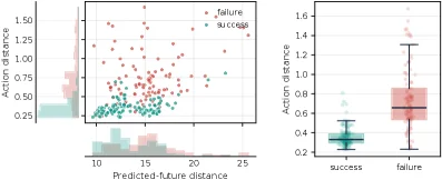
Figure 1 : Empirical motivation for world-action adversarial attacks. Failed episodes tend to have larger action shifts, while predicted-future shifts overlap across successful and failed executions. This motivates attacking the alignment between action and imagination.

This figure (Figure 1) serves as the empirical motivation section of the paper, aiming to explain why adversarial attacks on World-Action Models (WAMs) are necessary and what the targets of these attacks are.

First, let's look at the left chart. This is a scatter plot that combines the distribution of two variables: 1. X-axis: Labeled "Predicted-future distance". This variable represents the distance between the future state predicted by the model and a certain baseline (which could be a clean input or an expected state). We can understand it as the deviation between the "imagined" future by the model and the actual situation. 2. Y-axis: Labeled "Action distance". This variable represents the distance between the actually executed action and a certain baseline (which could be an optimal action or an expected action). We can understand it as the deviation between the "executed" action by the model and the desired action. 3. Data points: There are two colors of data points in the graph: * Red points represent "failure" episodes. * Turquoise points represent "success" episodes. 4. Distribution histograms: Below and to the left of the scatter plot, there are two histograms respectively: * The histogram below shows the distribution of "Predicted-future distance", where turquoise represents successful cases and red represents failed cases. * The histogram on the left shows the distribution of "Action distance". Similarly, turquoise represents successful cases and red represents failed cases.

From the left chart, we can observe: * For failed episodes (red points), their "Action distance" (Y-axis value) is generally larger. This means that in failed cases, the deviation between the action executed by the model and the desired action is greater. The histogram also shows that the distribution of action distances for failed cases is more biased towards larger values. * For successful episodes (turquoise points), their "Action distance" is relatively small. The histogram shows that the distribution of action distances for successful cases is more concentrated around smaller values. * Regarding "Predicted-future distance" (X-axis), the distributions of successful and failed episodes seem to overlap. This means that regardless of whether the episode is successful or failed, the deviation between the predicted future by the model and the baseline may not have a significant difference. The histogram also shows that there is a certain overlapping area in the distribution of predicted future distances for successful and failed cases.

Next, let's look at the right chart. This is a box plot used to compare the "Action distance" of successful and failed episodes: 1. X-axis: There are two categories, "success" and "failure". 2. Y-axis: It is also "Action distance". 3. Box plot elements: * The box represents the interquartile range (Q1 to Q3) of the data, and the line in the middle is the median. * The whiskers above and below the box usually represent the range of the data (for example, the farthest data points within 1.5 times the interquartile range). * The scattered points are outliers or all data points.

From the right box plot, we can see more clearly: * The box plot for the "failure" category shows that its median and overall distribution of "Action distance" are significantly higher than those of the "success" category. * The box plot for the "success" category shows that its "Action distance" is concentrated in a lower numerical range. * This further confirms the observation from the left graph: failed episodes tend to have larger action deviations.

The operational mechanism (empirical basis) revealed by this figure: This figure, through empirical data, shows a key difference in WAMs between failed and successful executions: failed executions are usually accompanied by larger action deviations, while the deviation of the predicted future does not have a significant difference between success and failure. This provides a clear entry point for adversarial attacks on WAMs. * Attack target: Since the root cause of failure lies in the disconnection between action execution and the expected (or imagined) future, especially the increase in action deviation, the attack can target this "alignment" relationship. * Attack strategy: The "world-action adversarial attacks" proposed in the paper are precisely aimed at disrupting this alignment between actions and imagination. Specifically: * Attackers can use small visual perturbations to make the model produce harmful action shifts. * There are two types of attacks: 1. Action-only attack: When attackers prioritize disruption, the attack will directly drive the model to execute actions that lead to task failure, which corresponds to increasing the "Action distance". 2. Imagination-preserving attack: When attackers also consider stealth, the attack will try to induce harmful action shifts while keeping the predicted future by the model (i.e., "Predicted-future distance") close to its clean imagination. This means that the attacker hopes that the model's "imagination" still looks reasonable, but its "action" deviates from the expectation.

Conclusion: By comparing the "action distance" and "predicted future distance" of successful and failed executions, this figure clearly shows that failed executions are associated with larger action deviations, while the deviation of the predicted future is not a key factor distinguishing success from failure. This provides empirical motivation for the attack method proposed in the paper: by attacking the alignment between actions and imagination, WAMs can be effectively made to fail, and even stealthy attacks can be achieved, where the model's imagination looks normal, but the action is wrong.

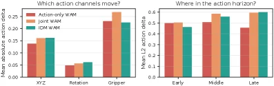
Figure 2 : Action-only adversarial attack produces structured action shifts. Across three WAM variants, the attack primarily perturbs continuous action channels and specific portions of the action horizon, rather than acting as uniform output noise.

This figure (Figure 2) clearly demonstrates how an "action-only adversarial attack" causes structured action shifts in World-Action Models (WAMs). It presents these findings through two side-by-side subfigures.

The left subfigure is titled "Which action channels move?". At its core, this chart shows which action channels are primarily affected by attacks across different types of WAM models. The horizontal axis lists three action channel types: "XYZ" (likely representing position or translation), "Rotation", and "Gripper". The vertical axis represents the "Mean absolute action delta", measuring the magnitude of action changes before and after the attack. The chart uses three colored bar graphs to represent three WAM variants: "Action-only WAM" (red), "Joint WAM" (orange), and "IDM WAM" (teal). From the data, it’s evident that attacks impact the "Gripper" channel most significantly, followed by the "XYZ" channel, while the "Rotation" channel is least affected. This indicates the attack isn’t random noise but selectively targets specific action dimensions.

The right subfigure is titled "Where in the action horizon?". This chart displays the distribution of attack impacts across different stages of an action sequence (i.e., along the action timeline). The horizontal axis is divided into three parts: "Early", "Middle", and "Late", representing different moments in the action sequence. The vertical axis shows the "Mean L2 action delta", also measuring the magnitude of action changes. Here too, three colored bar graphs represent the three WAM variants. The data reveals that for all three WAM variants, attacks have a stronger impact during the "Early" and "Late" stages of the action sequence, while their effect is relatively weaker in the "Middle" stage. This suggests the attack isn’t uniformly distributed across the action sequence but concentrates at specific time points.

Overall, this figure reveals the specific mechanism of the "action-only adversarial attack": rather than simply adding random noise to the model’s output, it produces structured action shifts. Specifically, this attack primarily affects certain action channels (e.g., gripper movements) and is more pronounced during specific parts of the action sequence (e.g., start and end phases). By comparing the responses of different WAM variants, we observe that despite variations, all models exhibit similar structured response patterns. This proves the attack’s effectiveness and target specificity, while also highlighting the vulnerability of WAMs to such attacks.

In summary, the figure’s conclusion is: For all three WAM variants, the action-only adversarial attack primarily disturbs continuous action channels (e.g., gripper and position) and specific parts of the action timeline (e.g., early and late phases), rather than acting as uniform output noise. This means the attack is structural, targeting key action outputs of the model.

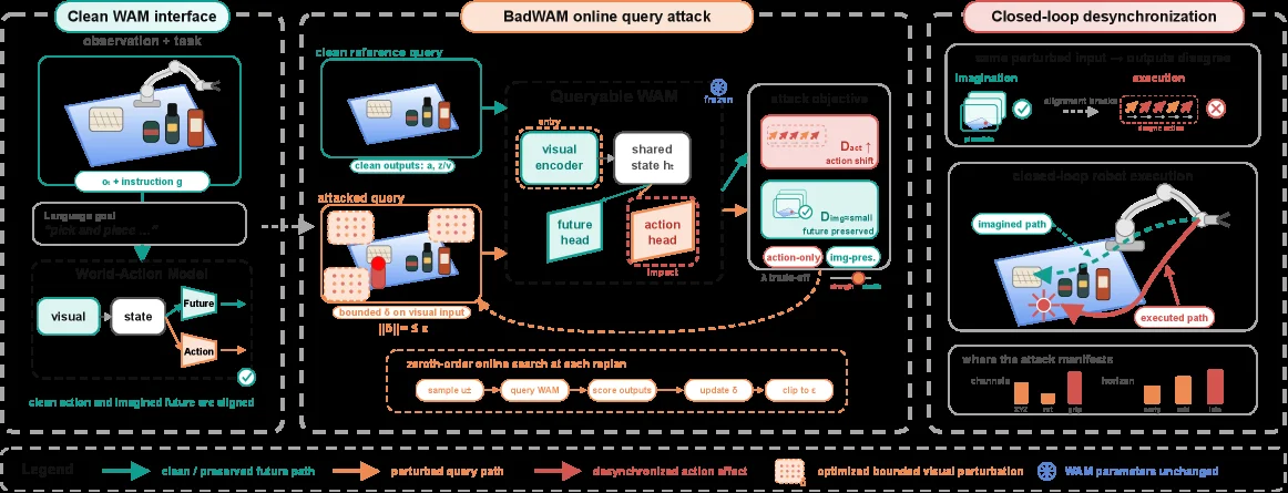
Figure 3 : Overview of BadWAM. BadWAM injects a small visual perturbation into model observations and performs query-based online search over a frozen WAM. The optimized trigger disrupts the action prediction pathway while preserving or minimally altering visual rollout predictions, leading to world-action adversarial attacks during closed-loop execution.

This diagram is an overview of the BadWAM method from the paper "BadWAM: When World-Action Models Dream Right but Act Wrong," clearly illustrating the entire process and core idea of the BadWAM attack.

First, look at the leftmost "Clean WAM interface" section, which shows the interface of a clean World-Action Model (WAM). In the upper part, the "observation + task" section has a diagram of a robot operation scene and an instruction \( g \), indicating that the input is a clean observation (such as a visual observation) and a task instruction. In the lower part, the "Language goal" and "World-Action Model" sections show the normal working process of WAM: visual input and state input enter WAM, and then WAM generates an action. At the same time, it imagines the future ("clean action and imagined future are aligned" means that the action and the imagined future are aligned at this time, that is, the model can correctly associate the action with its imagined future).

Next is the middle "BadWAM online query attack" section, which is the core part of the attack. The flow or information order is as follows: 1. First is the "clean reference query," where there is a clean observation (similar to the observation of the clean WAM on the left) and the corresponding clean output ("clean outputs: \( \hat{a}, \hat{z} \)", \( \hat{a} \) may be the clean action prediction, and \( \hat{z} \) is the clean future prediction). Then this clean query enters the "Queryable WAM" (a frozen WAM, that is, the parameters remain unchanged, and the icon of "WAM parameters unchanged" also explains this). 2. Then is the "attacked query," where a bounded perturbation is applied to the visual input ("bounded \( \delta \) on visual input", \( ||\delta|| \leq \epsilon \), \( \epsilon \) is a small upper limit of the perturbation), resulting in a perturbed visual input. This attacked query also enters the "Queryable WAM." 3. Inside the "Queryable WAM," there are a "visual encoder," a "shared state \( h \)" (shared state), a "future head" (used to predict the future), and an "action head" (used to predict the action). The attack objective is "attack objective," which has two parts: "\( D_{\text{act shift}} \) action shift" (action shift, hoping that the action deviates from the correct one) and "\( D_{\text{img small}} \) future preserved" (future preserved, hoping that the future prediction is close to the clean one, that is, to maintain or minimize the change in the visual roll-out prediction). There is "a trade-off" between these two objectives because both the action shift and the future preservation (or minimal change) need to be achieved at the same time. 4. Then there is the "zeroth-order online search at each timestep" (zeroth-order online search at each time step). The steps of this search process are: "sample \( \hat{u}_t \)" (sample the perturbation \( \hat{u}_t \)), "query WAM" (query WAM), "score outputs" (score the outputs), "update \( \delta \)" (update the perturbation \( \delta \)), "clip to \( \epsilon \)" (clip the perturbation to the range of \( \epsilon \)). Through this iterative process, the perturbation \( \delta \) is optimized to achieve the best attack effect.

Finally, the rightmost "Closed-loop desynchronization" section shows the performance of the attack in closed-loop execution: 1. In the upper part, the "Imagination" and "execution" sections: "Imagination" is the future imagined by the model (there is a green check mark, indicating that the imagined future seems reasonable), and "execution" is the actual executed action (there is a red cross, indicating that the actual executed action is wrong and inconsistent with the imagination). Here, "same perturbed input → output change" means that after the input is perturbed, the output (action) changes, resulting in a disconnection between imagination and execution. 2. In the middle, the "closed-loop robot execution" section shows the imagined path ("imagined path," green dashed line) and the actual executed path ("executed path," red solid line). It can be seen that the two are different, which is the action shift caused by the attack. 3. In the lower part, the "where the attack manifests" section is a bar chart showing the attack performance under different channels or categories. The orange and red bars represent different situations, indicating the effect of the attack in different cases.

In summary, the way the BadWAM method works is: inject a small visual perturbation into the observation of WAM, and then perform a query-based online search (zeroth-order search) on the frozen WAM to optimize this perturbation so that the action prediction path of WAM is disrupted (the action deviates from the correct one), but the visual roll-out prediction (imagined future) is preserved or minimally changed, thus leading to a world-action adversarial attack in closed-loop execution. That is, the future imagined by the model is reasonable, but the actual executed action is wrong, achieving a disconnection between the action and the imagination. There are two types of such attacks: one is the "action-only adversarial attack" that gives priority to disruption (directly driving the model to generate actions that lead to task failure), and the other is the "imagination-preserving adversarial attack" that gives priority to concealment (inducing harmful action shifts while keeping the future predicted by the model close to the cleanly imagined future). These two attacks cover the situation from open action hijacking to more hidden disconnection between action and imagination.

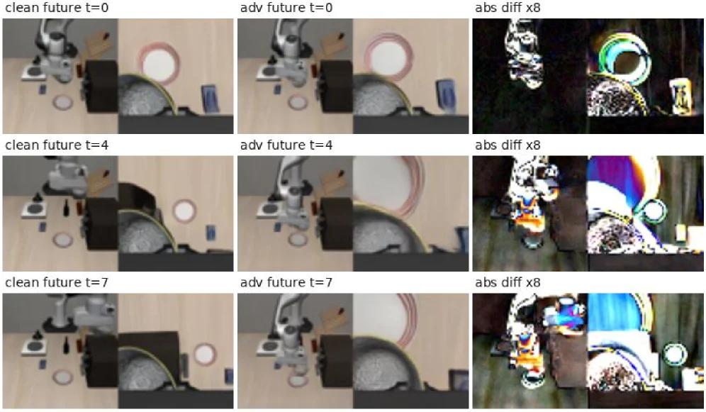
(a) Imagined future without preservation. (b) Imagined future with preservation. Figure 4 : Qualitative illustration of the imagination-preserving objective on IDM WAM. Each panel compares predicted futures under clean and adversarial observations at selected future steps. abs diff denotes the absolute pixel difference between clean and adversarial predictions, amplified by 8 × 8\times for visibility. Both variants induce action-space failure, but the preservation term keeps the adversarial future more consistent with the clean imagination.

This figure (Figure 4) provides a qualitative illustration of the "imagination preservation" objective in the IDM WAM model, aiming to demonstrate how the model's predicted future world states change under adversarial attacks.

First, let's examine the structure of the figure. It is organized into a 3x3 grid, where each row represents a specific "future step" (t=0, t=4, t=7). Each column represents different content: 1. First column (e.g., "clean future t=0"): This section shows the model's prediction of the future world without adversarial interference (i.e., "clean" input). Here, "clean future" refers to the future scenario predicted by the model based on the current state when it has not been attacked. For example, in the first row, first column, we see the model's imagination of the future at time step t=0, which is based on a clean observation. 2. Second column (e.g., "adv future t=0"): This section shows the model's prediction of the future world with adversarial interference. Here, "adv future" refers to the future scenario predicted by the model after being attacked (e.g., the input image is slightly perturbed). For example, in the first row, second column, we see the future imagined by the model at time step t=0 when faced with adversarial input. 3. Third column (e.g., "abs diff x8"): This section shows the absolute pixel difference between the "clean prediction" and the "adversarial prediction". To make these differences more apparent, the image is magnified by 8 times. "Abs diff" stands for absolute difference, highlighting the discrepancies between the two predicted images (clean and adversarial). For example, in the first row, third column, we can see the pixel-level differences between the clean prediction and the adversarial prediction at time step t=0.

Now, let's analyze the data flow and information presentation order in the figure: * Row direction (temporal dimension): From top to bottom (t=0, t=4, t=7), it shows how the model's predicted future states change over time. t=0 might represent an initial prediction step, while t=4 and t=7 represent subsequent future time points. This allows us to observe the evolution of the attack's effect over time. * Column direction (condition comparison): From left to right, the three columns within each row form a comparison group. First, look at the "clean prediction" in the first column, then the "adversarial prediction" in the second column, and finally the "difference image" in the third column. This layout enables readers to intuitively compare the differences in the model's predictions at the same time point, with and without an attack.

This figure reveals the specific workings of the method: * Core idea: The method (the "imagination preservation" objective in BadWAM) aims to study a specific type of adversarial attack that tries to induce the model to perform harmful actions without significantly altering the model's imagination of the future (i.e., the predicted world state). * Comparative display: By displaying the "clean prediction" and "adversarial prediction" side by side, we can observe whether the attack successfully changes the model's future imagination. If the adversarial prediction is very similar to the clean prediction (i.e., the differences in the difference image are small), it indicates that the attack is effective in "preserving imagination." * Difference visualization: The "abs diff x8" image in the third column is crucial as it quantifies and visualizes the extent of the attack's impact on the model's future imagination. If the color changes in the difference image are severe and widespread, it indicates that the attack has significantly disturbed the model's future predictions; conversely, if the differences are small, it indicates that the attack is effective in preserving imagination.

From the resulting figure, we can draw the following conclusions: * Coordinates and comparison objects: Each cell in the figure corresponds to a specific time step (t=0, t=4, t=7) and a prediction condition (clean or adversarial). The objects of comparison are the "clean prediction" and "adversarial prediction" at the same time step. * Main conclusion: According to the figure's caption, both variants (possibly referring to different attack methods or model configurations) led to failure in action space (i.e., the model took incorrect actions). However, the "preservation term" (imagination-preservation term) makes the adversarial future more consistent with the clean imagination. This means that when using the "imagination preservation" objective, even if the attack causes the model to take incorrect actions, the model's prediction of the future remains very similar to what it would be without an attack. In other words, the attack is "covert" because it does not obviously disrupt the model's imagination of the future but still leads to erroneous actions.

In summary, this figure, through qualitative comparison, shows how adversarial attacks affect the model's future predictions in the IDM WAM model, and how the "imagination preservation" objective ensures that the attack, while disrupting actions, maintains consistency in future predictions as much as possible. This makes the attack more covert because the model appears to still correctly imagine the future, yet it actually executes incorrect actions.

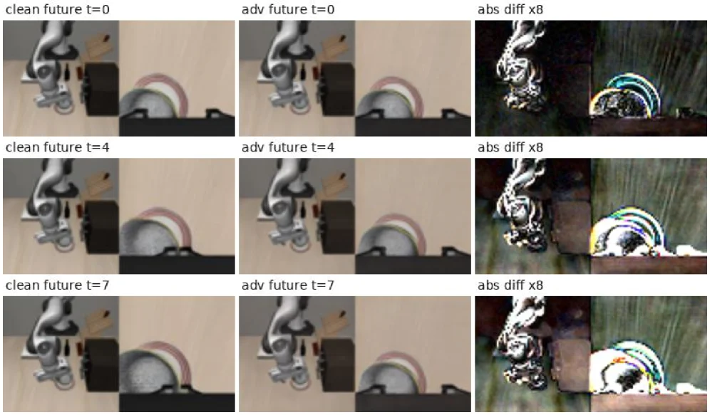
(a) Imagined future without preservation. (b) Imagined future with preservation. Figure 4 : Qualitative illustration of the imagination-preserving objective on IDM WAM. Each panel compares predicted futures under clean and adversarial observations at selected future steps. abs diff denotes the absolute pixel difference between clean and adversarial predictions, amplified by 8 × 8\times for visibility. Both variants induce action-space failure, but the preservation term keeps the adversarial future more consistent with the clean imagination.

This figure is a qualitative result display diagram used to intuitively illustrate the effect of the "imagination - preserving" objective on IDM WAM (a world - action model), and it is part of the content in the paper about the BadWAM attack evaluation.

Components of the Diagram and Information Flow

  • Meaning of Columns:
    • The first column (such as "clean future t = 0", "clean future t = 4", "clean future t = 7"): It shows the future scenarios predicted by the model when there is no adversarial perturbation (under clean observations). Here, "t" represents the time step (future step), and different t - values (0, 4, 7) correspond to different future time points. We can see the model's imagination (predicted world state) of the future when it is not attacked.
    • The second column (such as "adv future t = 0", "adv future t = 4", "adv future t = 7"): It shows the future scenarios predicted by the model when there is an adversarial perturbation (under adversarial observations), that is, the prediction results of the model after being attacked by BadWAM.
    • The third column ("abs diff x8"): It shows the absolute pixel difference between the clean prediction and the adversarial prediction, and this difference is magnified by 8 times ("x8") to make the difference more clearly visible. Through this difference diagram, we can intuitively see the degree of impact of the adversarial attack on the model's future prediction.
  • Meaning of Rows:
    • Each row corresponds to a specific future time step (t = 0, t = 4, t = 7). In this way, we can observe how the clean prediction, adversarial prediction, and their differences change at different time points.

How the Method Works (Logic Understood from the Diagram)

  • First, the model (here is IDM WAM) without adversarial situations (the first column) will predict the scenes of the future (different t - steps). These predictions show how the world state that the model originally "imagined" develops over time.
  • Then, when adversarial perturbations are applied (the second column), the model will predict the future based on the perturbed observations. We need to compare the difference between the adversarial prediction and the clean prediction (the absolute difference diagram in the third column).
  • From the diagram, we can see that the adversarial attack will cause changes in the model's future prediction (there are differences between the images in the second column and the first column). However, the "imagination - preserving" objective makes the adversarial future prediction (the second column) as close as possible to the clean future prediction (the first column) (visually, the difference between the image in the second column and the image in the first column is relatively small, especially in the case of "imagination - preserving"). At the same time, this attack still leads to failures in the action space (that is, there will be problems with the model's action execution, although its future imagination seems to be relatively close to the clean situation).

Comparison of Results and Conclusion

  • Objects of Comparison:
    • What is compared are the "clean future prediction" (the first column), the "adversarial future prediction" (the second column), and the pixel difference between them (the third column).
    • Comparison at different time steps (t = 0, t = 4, t = 7), so as to observe the effect of the attack at different time stages.
  • Conclusion:
    • Both attack variants (including the imagination - preserving attack) will lead to failures in the action space (that is, there will be problems with the model's action execution).
    • However, the "imagination - preserving" item (that is, the part of the adversarial attack that tries to preserve the model's future imagination) makes the adversarial future prediction (the second column) more consistent with the clean future prediction (the first column) (from the absolute difference diagram in the third column, we can see that the difference after the attack is relatively small, or in other words, after the model is attacked, its predicted future looks closer to what it originally imagined under clean conditions). In other words, even if the model is attacked and causes errors in action execution, from its future imagination, it seems to be relatively reasonable. This is where the stealth of the "imagination - preserving" attack lies — it can make the model's future imagination look fine, but the actions go wrong.

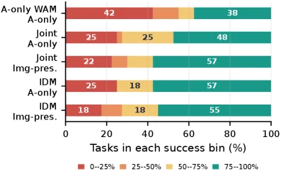
Figure 5 : Task-level failure profile under attack. Unlike Table 1 , which reports aggregate success, this figure shows how attacked tasks distribute across success-rate bins. Lower bins indicate tasks that are consistently broken rather than merely slightly degraded.

This figure (Figure 5) illustrates the distribution of tasks across various success rate intervals under different attack types. Unlike Table 1, which reports overall success rates, this graph focuses on how attacked tasks are distributed across different success "bins"—lower bins indicate tasks are consistently broken rather than just slightly degraded.

First, let's examine the axes and basic structure of the graph: * X-axis: Represents "Tasks in each success bin (%)", i.e., the percentage of tasks within each success rate interval. The range is from 0% to 100%. * Y-axis: Lists different attack types or model variants. From top to bottom, they are: * A-only WAM: Action-only World Action Model (possibly a baseline or specific variant). * Joint A-only: Jointly trained action-only model. * Joint Img-pres.: Jointly trained image-preservation model (possibly meaning the model tries to keep image predictions unchanged during attacks). * IDM A-only: Action-only version of some IDM (possibly referring to an image-action decoupled model or another specific model). * IDM Img-pres.: Image-preservation version of some IDM. * Color coding: The legend explains the success rate intervals represented by different colors: * Red (0--25%): Very low task success rate, almost always failing. * Orange (25--50%): Low task success rate, mostly failing. * Yellow (50--75%): Moderate task success rate, partly successful and partly failing. * Green (75--100%): Very high task success rate, almost always succeeding.

Next, we analyze the composition of each bar, which reveals the failure distribution of tasks under a specific attack type: 1. A-only WAM: The task distribution for this model is: 42% of tasks fall into the red region (0-25% success rate), a small number of tasks are in the orange (25-50%) and yellow (50-75%) regions, while 38% of tasks are in the green region (75-100% success rate). This indicates that under attack, a significant portion of tasks (42%) perform very poorly for this model, but nearly 40% of tasks still perform well. 2. Joint A-only: The task distribution for this model is more even: 25% in red, 25% in orange, and the remaining 50% (25% yellow + 48% green? Wait, no—each bar should sum to 100%. So it should be: 25% red, 25% orange, 25% yellow, and 48% green. This indicates that under attack, the failed tasks for this model are more widely distributed, from very poor to relatively good, but not as high a proportion of extremely poor tasks as with A-only WAM. 3. Joint Img-pres.: The task distribution for this model is: 22% red, a small amount of orange (value not labeled, but can be inferred), and then 57% green. This indicates that under "image-preservation" attacks, most tasks (57%) for this model still perform well, with only a few tasks (22%) performing very poorly. 4. IDM A-only: The task distribution for this model is: 25% red, 18% yellow, and 57% green. This indicates that under attack, a significant portion of tasks (25%) perform very poorly for this model, but most tasks (57%) still perform well. 5. IDM Img-pres.: The task distribution for this model is: 18% red, 18% yellow, and 55% green. This indicates that under "image-preservation" attacks, most tasks (55%) for this model still perform well, with 18% of tasks performing very poorly and another 18% performing moderately poorly.

What this figure reveals about the method's operation (or how attack effectiveness is evaluated): This figure evaluates the impact of different attacks on the performance of the WAM model by dividing tasks into four intervals based on their success rates and statistics the percentage of tasks falling into each interval under each attack type. This method allows us to intuitively see how attacks affect the model—are they causing most tasks to fail completely (a high proportion of red and orange regions), or just slightly degrading task performance (a high proportion of green regions, but with red regions possibly still present).

Conclusion: From the figure, it can be seen that different attack types have different impacts on the WAM model. For example, A-only WAM has a high proportion of tasks (42%) in the very low success rate interval (0-25%) under attack, indicating it is vulnerable to severe disruption. In contrast, the Joint Img-pres. and IDM Img-pres. models, under "image-preservation" attacks, have a high proportion of tasks (57% and 55% respectively) still in the high success rate interval (75-100%). This might mean these models are more capable of maintaining their functionality under attack, or that it is more difficult for attackers to completely fail tasks in these cases. Overall, this figure shows the distribution of task failure severities for the WAM model under different attack strategies, helping us understand the specificity of attacks and the robustness of the model.

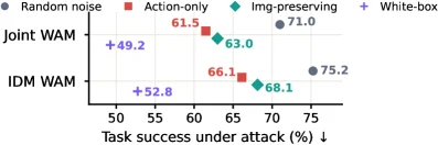
Figure 6 : Comparison with random perturbations on full LIBERO dataset. All methods use the same ℓ ∞ \ell_{\infty} budget. Lower task success indicates a stronger attack.

This figure is from the paper "BadWAM: When World-Action Models Dream Right but Act Wrong" and is used to compare the performance of different attack methods on the full LIBERO dataset, where all methods use the same ℓ∞ budget. A lower task success rate indicates a stronger attack.

Components of the Figure and Information Flow

  • X-axis: Labeled "Task success under attack (%) ↓", it represents the task success rate (in percentage) under attack. The downward arrow indicates that a smaller value (i.e., a lower task success rate) means a stronger attack.
  • Y-axis: Divided into two categories, "Joint WAM" and "IDM WAM", representing two different variants of the World-Action Model (WAM).
  • Data Points and Legend:
  • Blue dot (Random noise): Result of the random noise attack.
  • Red square (Action-only): Result of the action-only adversarial attack, which directly drives the model towards actions that lead to task failure.
  • Green diamond (Img-preserving): Result of the imagination-preserving adversarial attack, which tries to make the model's predicted future close to its clean imagination while inducing harmful action shifts.
  • Purple plus sign (White-box): Result of the white-box attack.
  • Numerical Labels: The numbers next to each data point (e.g., 49.2, 52.8, 61.5, etc.) are the corresponding task success rates (%). A smaller number indicates a stronger attack.

How the Methods Work (From the Figure)

  • We have three main attack methods to compare: random noise attack, action-only attack, imagination-preserving attack, and white-box attack as a reference.
  • For each WAM variant (Joint WAM and IDM WAM), we observe the task success rates under different attack methods:
  • In Joint WAM:
    • The task success rate of the random noise attack is 71.0%.
    • The task success rate of the action-only attack is 61.5%.
    • The task success rate of the imagination-preserving attack is 63.0%.
    • The task success rate of the white-box attack is 49.2%.
  • In IDM WAM:
    • The task success rate of the random noise attack is 75.2%.
    • The task success rate of the action-only attack is 66.1%.
    • The task success rate of the imagination-preserving attack is 68.1%.
    • The task success rate of the white-box attack is 52.8%.
  • From these data, we can see that the task success rates of both the action-only attack and the imagination-preserving attack are lower than that of the random noise attack, indicating that these two attacks targeting WAM are stronger than the random noise attack. And the task success rate of the white-box attack is the lowest, indicating that the white-box attack is the strongest among these attack methods. At the same time, the task success rate of the imagination-preserving attack is higher than that of the action-only attack (under the same WAM variant), which is consistent with the definition of the imagination-preserving attack: while inducing harmful action shifts, it tries to keep the model's predicted future close to the clean imagination, so its attack strength is relatively weaker than that of the action-only attack but still stronger than that of the random noise attack.

Conclusion

This figure shows the attack effects of different attack methods (random noise, action-only, imagination-preserving, white-box) on two WAM variants (Joint WAM and IDM WAM). The results show that specific adversarial attacks targeting WAM (action-only and imagination-preserving attacks) can reduce the task success rate more than the random noise attack. Among them, the white-box attack has the strongest effect, and the effect of the imagination-preserving attack is slightly weaker than that of the action-only attack but still stronger than that of the random noise attack. This verifies the effectiveness of the BadWAM framework proposed in the paper, that is, there are specific attacks targeting WAM, which can disrupt the alignment between the model's imagination and execution, thus reducing the task success rate.

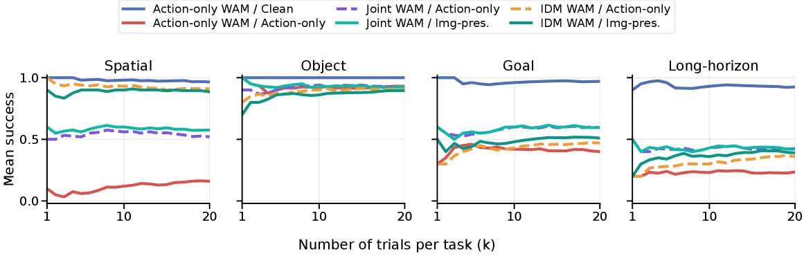
Figure 7 : Mean pass@ k k across trials on different LIBERO suites. BadWAM lowers success throughout the trial budget instead of only causing isolated unlucky failures.

This figure (Figure 7) is from the paper "BadWAM: When World-Action Models Dream Right but Act Wrong" and illustrates the average "pass@k" performance of models across different LIBERO task suites as the number of trials (in thousands, k) increases. Here, "pass@k" refers to the proportion (mean) of successful task completions within the first k trials, measuring the model's overall performance within a given trial budget.

The x-axis of the graph represents "Number of trials per task (k)", indicating the number of trials conducted for each task, ranging from 1k to 20k. The y-axis represents "Mean success", indicating the average probability of success, ranging from 0 to 1.

There are four subplots in the figure, corresponding to different task types: Spatial, Object, Goal, and Long-horizon. Each subplot contains multiple curves, with each curve representing a specific WAM (World-Action Model) variant and the attack or condition it faces:

  1. Solid blue line: Action-only WAM / Clean - This represents the performance of an Action-only WAM (which only learns action generation) in the absence of an attack (Clean). It serves as one of the baselines.
  2. Dashed purple line: Joint WAM / Action-only - This represents a Joint WAM (which learns both world prediction and action generation) subjected to an "action-only" type of attack.
  3. Dash-dotted orange line: IDM WAM / Action-only - This represents an IDM WAM (possibly a specific improvement or type of WAM) subjected to an "action-only" type of attack.
  4. Solid red line: Action-only WAM / Action-only - This represents an Action-only WAM subjected to an "action-only" attack. Note that this line performs very poorly, close to 0, in some tasks (e.g., Spatial and Long-horizon).
  5. Solid cyan line: Joint WAM / Img-pres. - This represents a Joint WAM subjected to an "image preservation" (Img-pres., possibly meaning maintaining consistency between imagined images and reality or the attack not affecting image imagination) type of attack.
  6. Solid dark green line: IDM WAM / Img-pres. - This represents an IDM WAM subjected to an "image preservation" type of attack.

Methodology revealed by the figure (Attack and Evaluation): This figure demonstrates the core idea of the BadWAM framework: introducing adversarial attacks against WAMs (BadWAM attacks) to disrupt the alignment between the "future world states" imagined by the WAM and the "actions" it actually executes. Specifically: - Attack Types: BadWAM defines two main types of attacks: * Action-only attack: This type of attack directly causes the model to take actions that lead to task failure, without considering whether its imagined future is reasonable. This is represented in the figure by curves labeled / Action-only (e.g., dashed purple line, dash-dotted orange line, solid red line). * Imagination-preserving attack: This type of attack attempts to induce harmful action shifts without significantly altering the model's imagination of the future world (i.e., preserving its "Img-pres."). This is represented in the figure by curves labeled / Img-pres. (e.g., solid cyan line, solid dark green line). - Evaluation Metric: The model's performance under different attacks is evaluated using "pass@k". If the model's performance decreases as the number of trials k increases, it indicates that the attack is effective. - WAM Variants: The figure compares the robustness of different types of WAMs (Action-only WAM, Joint WAM, IDM WAM) under different attacks.

Axes, Comparison Objects, and Conclusions: - Axes: The x-axis is the number of trials (k), and the y-axis is the mean success probability. - Comparison Objects: * Performance differences between different task types (Spatial, Object, Goal, Long-horizon). * Performance differences between different WAM variants (Action-only, Joint, IDM) for the same task type. * Performance differences of the same WAM variant under different attack types (Action-only vs. Img-pres.). * Performance differences before and after the attack (Clean vs. Attacked). - Conclusions: * From the figure, it can be seen that for most WAM variants and task types, the mean success probability (pass@k) of attacked models is generally lower than that of the unattacked baseline model (e.g., the solid blue line for Action-only WAM / Clean) as the number of trials increases. * This indicates that BadWAM attacks indeed effectively reduce model performance, and this reduction is consistent rather than being isolated unlucky failures occurring in only a few trials (as stated in the caption: "BadWAM lowers success throughout the trial budget instead of only causing isolated unlucky failures."). * Different WAM variants have varying sensitivities to attacks. For example, in the Spatial task, the Action-only WAM / Action-only (solid red line) performs very poorly, while the Action-only WAM / Clean (solid blue line) performs well. * "Imagination-preserving" attacks (Img-pres.) generally have a smaller impact on the performance of some WAM variants (e.g., Joint WAM and IDM WAM) compared to "action-only" attacks (Action-only), but this depends on the specific task and WAM type.

In summary, this figure visually demonstrates the effectiveness of BadWAM attacks by comparing the "pass@k" performance of different WAM variants under different attack types and tasks, showing that these attacks can consistently reduce the success rate of WAMs in various tasks, thus validating the hypothesis of WAM-specific failures proposed in the paper.

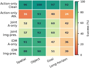
Figure 8 : Per-suite success rates on LIBERO. The attack is especially damaging on spatial and long-horizon tasks, while object-centric tasks remain comparatively more robust.

This figure (Figure 8) illustrates the attack effectiveness on the success rates of different types of "World-Action Models" (WAMs) using the LIBERO benchmark suite. Let's break down the figure step by step:

  1. Chart Structure and Components:

    • Y-axis (Rows): Represents different types of WAM models or their variants, listed from top to bottom:
      • Action-only Clean: This is likely a baseline model that only learns action prediction, without world state prediction, or its performance in a clean (unattacked) environment.
      • Action-only Atk.: This is a model under "action-only" attack. According to the paper, this type of attack directly drives the model to perform actions that lead to task failure.
      • Joint A-only: A joint model that might consider both actions and some form of "action-only" aspect of the attack or characteristics.
      • Joint Img-pres.: A joint model that might consider both actions and image presentation (i.e., world state prediction) aspects of the attack or characteristics.
      • IDM A-only: Likely refers to a specific type of WAM (e.g., based on an inverse dynamics model) under "action-only" attack.
      • IDM Img-pres.: Same as above, but under image presentation attack.
    • X-axis (Columns): Represents different task types in the LIBERO benchmark, listed from left to right:
      • Spatial: Spatial tasks, possibly involving object localization or navigation.
      • Object: Object-centered tasks, possibly involving object manipulation or recognition.
      • Goal: Goal-oriented tasks, possibly involving reaching a specific goal state.
      • Long-horizon: Long-horizon tasks, possibly requiring multi-step planning and execution.
    • Cell Color and Values: The number in each cell indicates the success rate (in percentage) for that specific model and task. The color coding also reflects the success rate: green indicates a high success rate (close to 100%), and red indicates a low success rate (close to 0%). The color bar on the right (ranging from red to green, labeled "Success (%)") provides the mapping between color and success rate.
    • Color Bar: Located on the right side of the chart, it shows the correspondence between colors and success rate percentages. Red represents a low success rate, and green represents a high success rate.
  2. How the Method Works (Inferred from the Figure):

    • This figure shows the impact of different attack methods on different WAM models across various tasks.
    • The Action-only Clean row serves as a baseline, showing the model's performance when unattacked.
    • The Action-only Atk. row shows that when the model is subjected to an "action-only" attack, its success rate drops significantly, especially on Spatial (16%) and Long-horizon (24%) tasks. This validates the destructive nature of the "action-only" attack mentioned in the paper.
    • Other rows (such as Joint A-only, Joint Img-pres., IDM A-only, IDM Img-pres.) show the performance of different WAM variants or under different attack strategies. For example, IDM A-only has a success rate of 91% on the Spatial task but only 36% on the Long-horizon task, indicating different robustness levels for different tasks.
    • By comparing the colors and values of different model rows for the same task type, one can evaluate the robustness of different attack methods or model architectures.
  3. Coordinates, Comparison Objects, and Conclusions:

    • Coordinates: The X-axis represents task types (Spatial, Object, Goal, Long-horizon), and the Y-axis represents model types.
    • Comparison Objects:
      • Performance of the same model across different tasks (e.g., Action-only Atk. on Spatial vs. Object tasks).
      • Performance of different models on the same task (e.g., Action-only Clean vs. Action-only Atk. on the Spatial task).
    • Conclusions:
      • As stated in the original caption: "Areas that are unclear or uncertain in the figure should be handled according to the caption or skipped; never output hesitations, self-questions, or self-corrections." However, based on the figure and caption, we can conclude:
      • Attacks are particularly destructive to Spatial (spatial) and Long-horizon (long-horizon) tasks, with their success rates significantly reduced under attack (e.g., Action-only Atk. is only 16% on the Spatial task).
      • In contrast, object-centered tasks (Object) are relatively more robust, with their success rates decreasing less under attack (e.g., Action-only Atk. is 93% on the Object task).
      • Different WAM variants also vary in their sensitivity to attacks. For example, IDM A-only maintains a high success rate (91%) on the Spatial task but a lower one (36%) on the Long-horizon task.

In summary, this figure visually demonstrates the impact of "world-action drift attacks" on different types of tasks by comparing the success rates of different WAM models after attacks. It confirms that attacks are more destructive to spatial and long-horizon tasks, while object-centered tasks are relatively more robust.

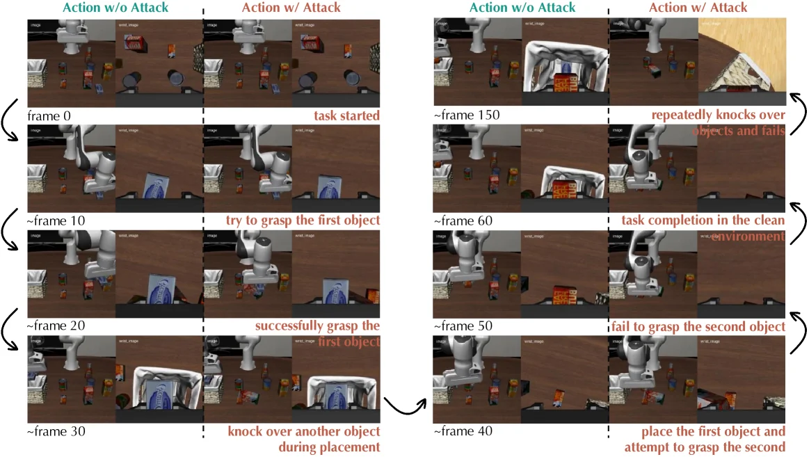
Figure 9 : Qualitative comparison of clean and attacked rollouts on a LIBERO-10 task. Each row shows synchronized third-person and wrist-camera observations over time. The clean WAM completes the sequential manipulation task, while the attacked WAM initially behaves plausibly but gradually drifts, knocks over objects, fails to grasp the second object, and eventually fails.

This figure qualitatively compares the rollouts of a clean (unattacked) World-Action Model (WAM) and an attacked WAM on a LIBERO-10 task, using synchronized third-person and wrist-camera observations over time. The image is divided into two main sections: the left side shows the "Action w/ Attack" (attacked WAM) and the right side shows the "Action w/o Attack" (clean WAM), each with a sequence of frames ordered by time.

Left Section: Attacked WAM ("Action w/ Attack")

  • Time-Ordered Frames: The frames are arranged vertically, from top to bottom, representing the progression of time: "frame 0", "~frame 10", "~frame 20", and "~frame 30". Each frame contains two synchronized views: a third-person perspective (left) and a wrist-camera perspective (right), showing the robot’s observation at that time.
  • Behavior Over Time:
  • At "frame 0" (task start), the robot is in its initial state with various objects around.
  • By "~frame 10", the robot attempts to grasp the first object ("try to grasp the first object").
  • By "~frame 20", the robot successfully grasps the first object ("successfully grasp the first object").
  • By "~frame 30", the robot knocks over another object during placement ("knock over another object during placement"), indicating the attack has started to disrupt behavior, causing deviation from the expected task trajectory.

Right Section: Clean WAM ("Action w/o Attack")

  • Time-Ordered Frames: Frames are ordered vertically: "~frame 40", "~frame 50", "~frame 60", and "~frame 150" (note the different frame numbering, reflecting a potentially faster/smoother execution for the clean model).
  • Behavior Over Time:
  • At "~frame 40", the robot places the first object and attempts to grasp the second ("place the first object and attempt to grasp the second").
  • By "~frame 50" (annotation may have a typo; context suggests successful grasping here, as the task completes later).
  • By "~frame 60", the robot completes the task in the clean environment ("task completion in the clean environment").
  • "~frame 150" shows repeated object knockovers and failure for the attacked model (contextual contrast).

Arrows and Annotations

  • Arrows: Black arrows (left and right) indicate the flow of time, guiding the viewer through the sequence of actions.
  • Red Annotations: These explain the robot’s behavior at each frame (e.g., "try to grasp the first object", "successfully grasp the first object", "knock over another object during placement" for the attacked model; "task completion in the clean environment" for the clean model).

Revealing the Attack’s Impact

  • The attacked WAM initially behaves plausibly (e.g., grasping the first object) but gradually drifts: it knocks over objects, fails to grasp the second object, and ultimately fails.
  • The clean WAM completes the task without errors.
  • This contrast shows that small visual perturbations (attacks) break the alignment between the WAM’s imagined future and its executed actions, causing behavior to shift from seemingly reasonable to failure.

In summary, the figure uses time-sequenced, synchronized observations to compare the attacked and clean WAMs, demonstrating how BadWAM attacks disrupt the model’s action-future prediction alignment, leading to task failure.

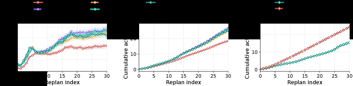
Figure 10 : Per-replan action shifts persist across execution and accumulate over time, with failed episodes showing substantially larger cumulative shifts than successful ones. Action shift is measured between clean and attacked action chunks at each replan; shaded regions denote 95% confidence intervals.

This figure (Figure 10) illustrates the dynamic changes in action shifts within World-Action Models (WAMs) during execution and their accumulation over time when under attack. We can understand its content and the method's operation from three subplots:

First, let's examine the leftmost subplot, which is a line graph. The x-axis is "Replan index," representing the number or step of replanning during execution; the y-axis is "Action shift (Δa)," indicating the difference between the attacked action chunk and the clean (unattacked) action chunk at each replanning step. There are four lines of different colors, each representing different types of experiments or model variants (according to the legend, possibly including different attack types or model configurations). The points on each line and their surrounding shaded regions (according to the caption, 95% confidence intervals) show the average action shift and its statistical fluctuation range at that replanning step. From the graph, it is evident that the action shift generally shows an increasing trend as the number of replans increases, with different variants exhibiting varying rates of growth and final shift magnitudes.

The middle subplot is a cumulative plot, with the x-axis also being "Replan index" and the y-axis being "Cumulative action shift." This graph demonstrates how the action shift accumulates over time (i.e., as the number of replans increases). There are two main curves, one in red and one in cyan (possibly representing failed and successful episodes, or different types of attacks). Both curves show a clear upward trend, indicating that the action shift continues to accumulate. The red curve (possibly representing failed episodes) has a significantly higher cumulative shift than the cyan curve (possibly representing successful episodes), consistent with the caption's description that failed episodes exhibit substantially larger cumulative shifts.

The rightmost subplot is also a cumulative plot, similar in structure to the middle one, but the specific shape and numerical range of the curves may differ. It similarly shows the growth of cumulative action shift with an increasing number of replans, where one curve (e.g., red) has a faster growth rate and a larger final cumulative shift than the other curve (e.g., cyan), further confirming that the accumulation effect of action shifts is more pronounced in failed episodes.

Combining these three subplots, we can draw the following conclusions: 1. Action shifts persist during execution and accumulate over time (as the number of replans increases). 2. The cumulative action shift in failed episodes is significantly larger than in successful episodes, indicating that the accumulation of action shifts is a crucial factor leading to task failure. 3. By analyzing the dynamics of action shifts under different model variants or attack types, we can better understand the behavioral patterns and vulnerabilities of WAMs when under attack.

This figure reveals how the BadWAM attack affects WAMs: the attack introduces small visual perturbations that disrupt the alignment between the model's action generation and future world prediction. This disruption manifests as persistent and accumulating action shifts, ultimately potentially leading to task failure. By comparing the cumulative action shifts in failed and successful episodes, the impact of this attack can be quantified.

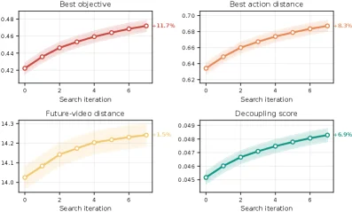
Figure 11 : Search dynamics for the imagination-preserving attack. Each panel uses a metric-specific y-axis range and reports mean ± \pm 95% confidence interval across replans. The query-based optimizer consistently improves the objective and increases action deviation, while the future-video distance changes much less in relative terms.

This figure (Figure 11) illustrates the search dynamics for an "imagination-preserving attack," consisting of four subplots. Each subplot displays a specific metric's change over "Search iteration." The metrics are: Best objective, Best action distance, Future-video distance, and Decoupling score. The x-axis in each subplot represents "Search iteration," ranging from 0 to 6, indicating different stages of the optimization process.

  1. Top-left subplot: "Best objective"

    • Content: This subplot shows the change in the "best objective" value during the search process. The y-axis range is approximately between 0.42 and 0.48.
    • Trend: As the number of search iterations increases (from 0 to 6), the best objective value shows a clear upward trend (red curve). This indicates that the optimizer is continuously improving the objective, moving it towards a more optimal direction. The figure also marks "-11.7%," which likely refers to the percentage improvement relative to a baseline (e.g., initial state or unattacked state).
    • Implication: This suggests that the attack optimizer successfully found an action sequence that increased the "objective," although this "objective" might have a specific meaning in the context of the attack (e.g., it could be a manipulated target rather than the task's original intended target).
  2. Top-right subplot: "Best action distance"

    • Content: This subplot shows the change in "best action distance" during the search process. The y-axis range is approximately between 0.62 and 0.70.
    • Trend: As the number of search iterations increases, the best action distance also shows an upward trend (orange curve). This indicates that the attack causes the model's actions to diverge more from a reference action (e.g., actions in a clean state or expected actions).
    • Implication: This directly reflects the effect of the attack, meaning the model's executed actions are deviating from what they should originally be. The figure also marks "-9.3%," which likely refers to the percentage increase in action distance relative to a baseline.
  3. Bottom-left subplot: "Future-video distance"

    • Content: This subplot shows the change in "future-video distance" during the search process. The y-axis range is approximately between 14.0 and 14.3.
    • Trend: As the number of search iterations increases, the future-video distance also increases (yellow curve), but the magnitude of change is relatively small.
    • Implication: This metric measures the difference between the model's predicted future world state and a reference future (e.g., future predictions in a clean state). A characteristic of the "imagination-preserving attack" is to keep the model's imagination (prediction) of the future close to the state before the attack, so the relatively small change in this metric aligns with the definition of the attack. The figure also marks "-1.5%," which likely refers to the percentage increase in future-video distance relative to a baseline.
  4. Bottom-right subplot: "Decoupling score"

    • Content: This subplot shows the change in "decoupling score" during the search process. The y-axis range is approximately between 0.045 and 0.049.
    • Trend: As the number of search iterations increases, the decoupling score shows an upward trend (cyan curve). The decoupling score might measure the degree of coupling between action generation and future prediction, or the extent to which the attack successfully induces action deviation.
    • Implication: An increase in this score might indicate that the attack has, to some extent, successfully altered the relationship between actions and predictions, or increased the degree of action deviation. The figure also marks "+6.9%," which likely refers to the percentage increase in the decoupling score relative to a baseline.

Revealing the Method's Operation: This figure reveals the specific operation of the "query-based optimizer" in the "imagination-preserving attack" by showcasing its performance. The optimizer's goal is to induce harmful action deviations from the model while keeping its future predictions (imagination) relatively stable. * Objective Improvement: The increase in the "best objective" indicates that the optimizer is effectively searching for actions that meet a specific optimization goal (possibly defined by the attacker). * Action Deviation: The increase in "best action distance" indicates that the optimizer successfully made the model's actions deviate from the expected or clean path. * Imagination Preservation: The relatively small change in "future-video distance" validates the characteristic of the "imagination-preserving attack," meaning the attack tries not to affect the model's ability to imagine the future, thus making it more covert. * Decoupling Effect: The increase in the "decoupling score" might indicate that the attack has introduced a greater difference between actions and future predictions, or that the attack's success is higher.

Coordinates, Comparison Objects, and Conclusion: * Coordinates: The x-axis in all subplots is "Search iteration," ranging from 0 to 6. The y-axis in each subplot represents a different metric, with ranges as described above. * Comparison Objects: The curves in each subplot represent the average performance across multiple "replans" at different search iterations, along with their 95% confidence intervals. Therefore, the curves show the average trend of each metric as the search iteration progresses. * Conclusion: This figure clearly shows that the proposed query-based optimizer is effective in the "imagination-preserving attack." It can continuously improve the attack objective, increase action deviation, while keeping the model's future predictions (imagination) relatively stable (i.e., the future-video distance does not change much). This indicates that the method can successfully induce the model to perform harmful actions without significantly disrupting its imagination ability, thus achieving the purpose of the "imagination-preserving attack." The percentage changes in the figure (e.g., -11.7%, -9.3%, -1.5%, +6.9%) further quantify the extent of these changes.

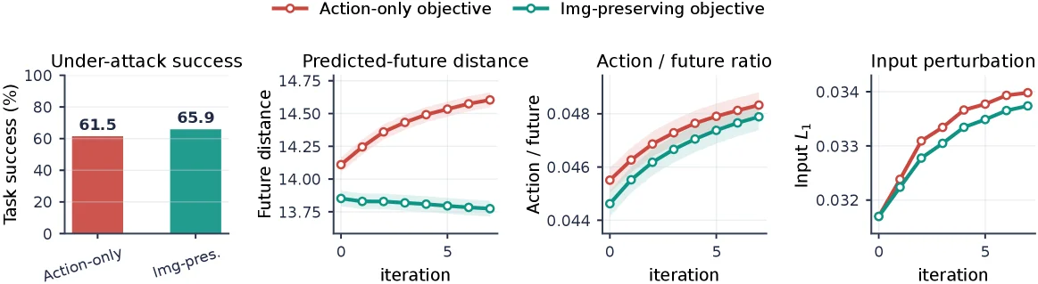
Figure 12 : Matched-strength stealth trade-off. The imagination-preserving objective produces consistently smaller predicted-future shifts under a comparable input perturbation budget, revealing a stealthier failure mode than the action-only objective. Shaded regions denote 95% confidence intervals over replans.

This figure (Figure 12) presents key results from the "Concealment Trade-off in Matching Strength" experiment, designed to compare the performance of two different attack objectives (Action-only objective and Image-preserving objective) under adversarial attacks. Specifically, it examines how these objectives affect the alignment between a model's predicted future and its actual executed actions, as well as which objective is more concealed when the input perturbation budget is comparable.

The figure consists of four subplots, each illustrating different evaluation metrics from left to right:

  1. First Subplot (Far Left): "Under-attack success" (Task Success Rate Under Attack)

    • This is a bar chart comparing the task success rates (in percentage) of two attack objectives—Action-only (red) and Img-preserving (green)—when the attack is successful.
    • The red bar represents the Action-only objective, with a task success rate of 61.5%.
    • The green bar represents the Img-preserving objective, with a task success rate of 65.9%.
    • This chart shows that the Img-preserving objective achieves a slightly higher task success rate under attack compared to the Action-only objective, though this may not be the primary metric for measuring concealment but rather provides a baseline comparison.
  2. Second Subplot: "Predicted-future distance"

    • This is a line graph with "iteration" on the x-axis and "Future distance" on the y-axis.
    • The red line represents the Action-only objective; as the number of iterations increases (from 0 to 5), the predicted future distance significantly increases, rising from approximately 14.0 to over 14.5.
    • The green line represents the Img-preserving objective; its predicted future distance remains relatively stable throughout the iterations, fluctuating between approximately 13.75 and 13.85, which is much lower than the red line.
    • This chart reveals the impact of the two attack objectives on the model's predicted future: the Action-only attack causes a substantial change in the model's predicted future (increased distance), while the Img-preserving attack better maintains the model's predicted future close to its original (clean) state (minimal distance change).
  3. Third Subplot: "Action / future ratio"

    • This is also a line graph, with "iteration" on the x-axis and "Action / future ratio" on the y-axis.
    • The red line represents the Action-only objective, and the green line represents the Img-preserving objective.
    • As the number of iterations increases, the action/future ratio for both objectives rises, but the red line (Action-only) consistently remains slightly higher than the green line (Img-preserving).
    • This ratio likely reflects the degree to which the attack affects the relationship between the action and the future prediction. A higher ratio may indicate poorer alignment between the action and the future prediction.
  4. Fourth Subplot: "Input perturbation"

    • This is a line graph with "iteration" on the x-axis and "Input L₁" (a measure of input perturbation magnitude) on the y-axis.
    • The red line represents the Action-only objective, and the green line represents the Img-preserving objective.
    • As the number of iterations increases, the input perturbation for both objectives increases, but the red line (Action-only) shows slightly greater perturbation than the green line (Img-preserving).

How the Method Works (Inferred from the Figure): This figure illustrates a comparative experiment where researchers designed two types of adversarial attacks targeting World-Action Models (WAMs): * Action-only objective: This attack directly targets the model's action generation component, aiming to make the model execute actions that lead to task failure, without much concern for whether the model's future prediction aligns with the original prediction. This is evident in the "Predicted-future distance" graph, where this objective's attack causes a significant increase in the predicted future distance. * Image-preserving objective: This attack attempts to make the model execute harmful actions while trying to keep its future prediction close to the original (unattacked) prediction. This is reflected in the "Predicted-future distance" graph, where this objective's attack results in minimal change to the predicted future distance.

The experiment applies these attacks over multiple iteration steps, evaluating different metrics at each step.

Conclusion: Based on the data in the figure, the following conclusions can be drawn: * When an attacker prioritizes concealment (using the image-preserving objective), the change in the model's predicted future ("Predicted-future distance") is much smaller for a comparable input perturbation budget (as seen in the "Input perturbation" graph, where the perturbation levels for both objectives are similar, or the image-preserving objective's perturbation is slightly smaller). This means the image-preserving objective's attack is a more concealed failure mode because the model appears to still be imagining a reasonable future, yet it executes harmful actions that are misaligned with that imagination. * In contrast, the Action-only objective's attack, while also leading to an increase in task success rate (in the first subplot), significantly alters the model's predicted future, making its failure mode more apparent (less concealed). * The shaded regions in the figure represent 95% confidence intervals, indicating that these results are averages from multiple replans with statistical uncertainty.

In summary, this figure clearly demonstrates the advantage of the image-preserving objective's adversarial attack over the action-only objective's attack in maintaining alignment between the model's predicted future and its actual executed actions, thereby revealing a more concealed WAM-specific failure mode.

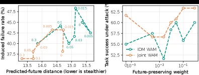
Figure 13 : Ablation on future-preserving weight λ \lambda . Moderate future preservation can improve the action-future tradeoff, while excessive preservation weakens action manipulation.

This image contains two subplots illustrating the impact of the future-preserving weight (λ) on model performance, focusing on the trade-off between "future preservation" and "action manipulation." Here's a detailed breakdown of each section:

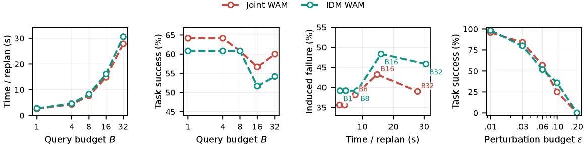
Figure 14 : Efficiency and budget sensitivity of BadWAM. Increasing the query budget B B raises the per-replan optimization cost, but also gives the optimizer more opportunity to find stronger perturbations. The perturbation-budget study further shows that larger ϵ \epsilon consistently improves attack effectiveness. Together, the curves expose the practical tradeoff among attack strength, stealthiness, and runtime.

This figure (Figure 14) is from the paper "BadWAM: When World-Action Models Dream Right but Act Wrong" and illustrates the efficiency and budget sensitivity of the BadWAM attack method. We can break this figure down into four subplots, which we will analyze from left to right:

The first subplot (farthest to the left) has the x-axis labeled "Query budget B," representing the number of queries an attacker can make during each replanning session. The y-axis is labeled "Time / replan (s)," indicating the computational time required for each replanning. There are two curves here, representing the "Joint WAM" and "IDM WAM" models. As the query budget B increases (from 1 to 32), the time required for each replanning significantly increases. This suggests that increasing the query budget raises the optimization cost per replanning (longer computation time) but also gives the optimizer more opportunities to find stronger perturbations (since more queries mean more information or attempts).

The second subplot also has the x-axis labeled "Query budget B," while the y-axis is labeled "Task success (%)." This subplot shows the task success rate under different query budgets. The two curves correspond to different models or attack scenarios (possibly indicating whether the attack successfully causes the task to fail). As the query budget increases, the task success rate fluctuates, but there is no clear monotonic trend overall. This might suggest that increasing the query budget within a certain range can improve attack effectiveness (lowering task success rate), but beyond a certain point, the effect may stabilize or change little.

The third subplot has the x-axis labeled "Time / replan (s)" and the y-axis labeled "Induced failure (%)." It shows the induced failure rate under different replanning times. The plot includes labeled points such as B8, B16, and B32, which likely represent different query budgets. As the replanning time increases, the induced failure rate first increases, then decreases, and then slightly increases again. This indicates that there is an optimal replanning time that maximizes the induced failure rate. This also validates the conclusion of the first subplot: increasing the query budget (and thus the replanning time) can enhance attack effectiveness, but beyond a certain time, the effect may diminish.

The fourth subplot has the x-axis labeled "Perturbation budget ε," representing the maximum amount of perturbation an attacker can apply to the input image. The y-axis is labeled "Task success (%)." There are two curves here, representing different models or attack scenarios. As the perturbation budget ε increases (from 0.01 to 0.20), the task success rate significantly decreases. This shows that a larger perturbation budget significantly improves attack effectiveness (making it easier to cause task failure).

Combining these four subplots, we can draw the following conclusions: 1. Increasing the query budget B raises the computational time per replanning but also gives the optimizer more opportunities to find stronger perturbations, thereby enhancing attack effectiveness. 2. There is an optimal replanning time that maximizes the induced failure rate, reflecting a trade-off between attack strength, stealth, and runtime. 3. Increasing the perturbation budget ε significantly improves attack effectiveness, leading to a decrease in task success rate.

This figure reveals how the BadWAM attack method operates by showing the impact of different budgets (query budget and perturbation budget) on attack effectiveness (task success rate, induced failure rate) and computational time. It demonstrates that attackers can balance attack strength, stealth, and runtime by adjusting these budgets to achieve the best attack outcomes.

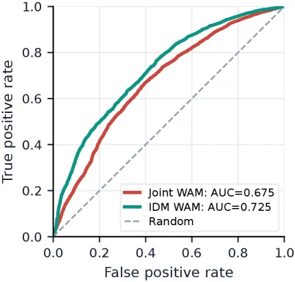
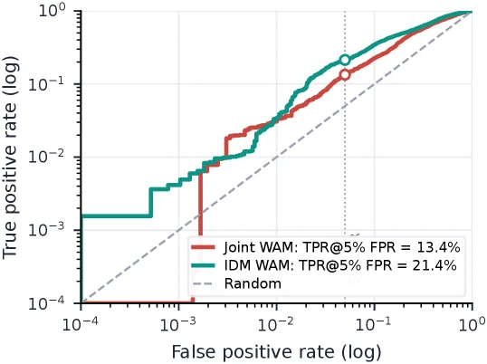
Figure 15 : Augmentation-consistency detection is insufficient against imagination-preserving attacks.

This diagram is a Receiver Operating Characteristic (ROC) curve, used to compare the performance of different models under the "enhanced consistency detection" method, thereby illustrating the limitations of this approach in countering "imagination-preserving attacks."

Explanation of Components in the Diagram:

  • Horizontal Axis (X-axis): Represents the False Positive Rate, which is the proportion of normal cases incorrectly classified as abnormal. The range is from 0 to 1, with higher values indicating more false alarms.
  • Vertical Axis (Y-axis): Represents the True Positive Rate, which is the proportion of abnormal cases correctly classified as abnormal. The range is from 0 to 1, with higher values indicating better detection performance.
  • Curves:
  • Red Curve: Represents the ROC curve for the "Joint WAM" model, with an AUC (Area Under the Curve) of 0.675. The closer the AUC value is to 1, the better the model's classification performance.
  • Green Curve: Represents the ROC curve for the "IDM WAM" model, with an AUC of 0.725.
  • Dashed Line: Represents the "Random" (random guessing) scenario, with an AUC of 0.5. This line serves as a benchmark, and the ROC curve of any effective detection method should lie above it.
  • Legend: Located at the bottom right of the diagram, it labels each curve with the corresponding model name and its AUC value.

How the Method Works:

This diagram demonstrates the performance of the "enhanced consistency detection" method across different WAM models. The core idea of this method is to determine the presence of an attack by detecting the consistency between the future world state predicted by the model and the actual executed action. However, the results in the diagram indicate that even under "imagination-preserving attacks," the detection performance of this method remains limited.

Result Analysis:

  • Comparison Subjects: The diagram compares three scenarios: two different WAM models (Joint WAM and IDM WAM) and a random guessing scenario.
  • Conclusion: From the diagram, it is evident that the ROC curves of both WAM models lie above the random guessing line, indicating that the "enhanced consistency detection" method can detect attacks to some extent. However, the AUC values of both curves are below 0.8, suggesting that the detection performance is not ideal. Particularly, when facing "imagination-preserving attacks," this method may not be sufficient to effectively distinguish between normal situations and attack scenarios. Therefore, the results in the diagram indicate that the "enhanced consistency detection" method has limitations in countering "imagination-preserving attacks."

In summary, this diagram visually presents the performance of the "enhanced consistency detection" method across different WAM models through ROC curves and reveals its limitations in combating "imagination-preserving attacks."

Figure 15 : Augmentation-consistency detection is insufficient against imagination-preserving attacks.

This figure is a Receiver Operating Characteristic (ROC) curve, used to compare the performance of different methods in detecting a specific type of attack (here, "imagination-preserving attacks"). We can understand it through the following components:

  1. Axes:

    • X-axis (Horizontal): Represents the "False Positive Rate (FPR)" on a logarithmic scale (log scale). FPR measures the proportion of negative instances that are incorrectly classified as positive. The logarithmic scale allows for a clearer view of performance differences in the low FPR region. The range is from \(10^{-4}\) to \(10^0\).
    • Y-axis (Vertical): Represents the "True Positive Rate (TPR)" also on a logarithmic scale (log scale). TPR measures the proportion of positive instances that are correctly classified as positive, also known as "recall" or "sensitivity." The range is from \(10^{-4}\) to \(10^0\).
  2. Curves and Comparisons:

    • Red Curve (Joint WAM): Represents the performance of a method or model named "Joint WAM."
    • Green Curve (IDM WAM): Represents the performance of another method or model named "IDM WAM."
    • Dashed Line (Random): This is a diagonal dashed line representing the performance of a random guessing strategy. In an ROC curve, random guessing would lie along the diagonal line from \((0,0)\) to \((1,1)\) (or a similar slope on a log scale). Any effective detection method's curve should lie above this line; the further it is from the line, the better its performance.
  3. Key Data Points and Conclusion:

    • The figure marks two specific points on the curves, corresponding to the True Positive Rate (TPR) of each method when the False Positive Rate (FPR) is 5% (approximately \(10^{-1.3}\) on the log scale, indicated by vertical dashed lines).
    • For "Joint WAM" (red curve), at an FPR of 5%, its TPR is 13.4%. This point is marked with an empty circle.
    • For "IDM WAM" (green curve), at an FPR of 5%, its TPR is 21.4%. This point is also marked with an empty circle.
    • Conclusion: From the graph, it is evident that at the same low FPR of 5%, "IDM WAM" has a higher TPR (21.4%) than "Joint WAM" (13.4%). This means "IDM WAM" performs better in detecting this type of attack compared to "Joint WAM."
    • The original title, "Augmentation-consistency detection is insufficient against imagination-preserving attacks," suggests that both methods might be based on an "augmentation-consistency detection" strategy. However, the results of this figure indicate that even with this strategy, different implementations (like Joint WAM and IDM WAM) exhibit significant differences in performance against "imagination-preserving attacks." Specifically, while both attempt to detect attacks, IDM WAM shows greater effectiveness against this particular type of attack.

In summary, this figure compares the performance of two different WAM methods using an ROC curve, demonstrating their ability to detect "imagination-preserving attacks." The results show that, under the same FPR, IDM WAM can detect more true attacks (i.e., has a higher TPR), thus indicating stronger robustness against this type of attack.

← → flip · ↑ ↓ scroll notes · Esc exit