🌊 Tide

Information moves like the tide. We pick the waves worth studying.

中文

← Today's tide

Published 2026-07-08 · BytedTsinghua-SIA · Shiyuan Feng, Huan-ang Gao, Haohan Chi et al.

Weak-to-Strong Generalization via Direct On-Policy Distillation

arXiv · HuggingFace · ▲131

Abstract (verbatim)

Reinforcement learning with verifiable rewards (RLVR) is a powerful recipe for improving language-model reasoning, but it is expensive to repeat on every new strong model because the target model must generate many rollouts during training. As models scale, post-training itself becomes a bottleneck. We study a weak-to-strong alternative: run RL on a smaller model where rollouts are cheaper, then reuse what that RL run learned to improve a stronger target model. Directly distilling the post-RL weak teacher is not enough, because the teacher's final policy mixes useful RL gains with the limitations of the smaller model. We propose Direct On-Policy Distillation (Direct-OPD), which transfers the teacher's RL-induced policy shift instead. Direct-OPD compares the post-RL teacher with its own pre-RL reference and treats their log-ratio as a dense implicit reward for the student. In plain terms, the checkpoint pair tells us which actions RL made the weak model more or less likely to take, and Direct-OPD applies that signal on the stronger student's own on-policy states. This directly reuses the weak model's RL supervision signal without running sparse-reward RL on the target model. Empirically, Direct-OPD consistently leverages weaker teachers to improve stronger target models; notably, it boosts Qwen3-1.7B from 48.3% to 58.3% on AIME 2024 in just 4 hours on 8 A100 GPUs. It outperforms step-matched direct RL and enables the sequential composition of multiple policy shifts. Our results show that RL outcomes can be reused across model scales as implicit reward signals, not merely as final models to imitate.

Background

Background Analysis

1. Technical Context and Need
Recently, reinforcement learning with verifiable rewards (RLVR) has become a dominant method for enhancing reasoning in large language models (e.g., DeepSeek-R1, JustRL). The core idea is to train models by generating behaviors (rollouts), receiving feedback, and optimizing policies in an environment. However, this approach faces a significant bottleneck: larger models are more computationally expensive to train—generating behaviors slows down, and each RL iteration becomes costlier. As models scale, retraining RLVR from scratch for every new strong model becomes impractical, creating a need for more efficient post-training methods.

2. Limitations of Previous Methods
Traditional approaches directly imitate the final policy of a weak model (e.g., "policy distillation"), but this has fundamental flaws: the weak model’s final policy mixes useful improvements from RL with its inherent limitations. For example, when the target model (student) is already stronger than the weak model, imitating the weak model’s policy may overwrite the student’s superior behaviors (as shown in Figure 1(a), where a strong model is dragged down by the weak model’s policy). Additionally, running RL directly on strong models is expensive, and existing methods cannot reuse the supervisory signals learned during the weak model’s RL training.

3. Proposed Solution
The paper introduces "Direct On-Policy Distillation (Direct-OPD)," which focuses on transferring the "policy shift" induced by RL in the weak model, rather than the weak model itself. Specifically, by comparing the weak model’s behavior before and after RL training (i.e., "policy shift"), it extracts the supervisory signal from RL’s modifications and applies this signal as an implicit reward to train a stronger model (student). This avoids rerunning RL on the strong model while preserving the effective supervision from the weak model’s RL training. Experiments show that this method significantly improves strong models’ performance (e.g., Qwen3-1.7B’s score on AIME 2024 rises from 48.3% to 58.3%) with only a fraction of the cost of direct RL.

4. Key Differences from Prior Work
Unlike traditional policy distillation, Direct-OPD does not rely on the weak model’s final policy but focuses on the "policy shift," a more essential supervisory signal. Additionally, it does not require explicit reward model training or high overlap between the weak and strong models, enabling effective transfer across scales and reasoning patterns. This approach transforms RL’s outcomes from "single-model optimization" to "reusable cross-scale signals," offering a new direction for efficient post-training of large models.
Method, Figure by Figure

M E T H O D1 / 14

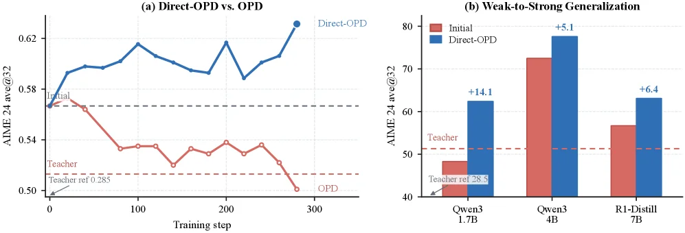
Figure 1 : Direct-OPD transfers the effect of small-model RL rather than imitating the small model. (a) Starting from R1-Distill-7B, vanilla OPD toward the post-RL JustRL-1.5B teacher degrades performance, whereas Direct-OPD transfers the JustRL-1.5B − - R1-Distill-1.5B policy shift and improves the student. (b) The same policy shift improves Qwen3-1.7B, Qwen3-4B, and R1-Distill-7B on AIME 2024, including students whose initial accuracy already exceeds the post-RL teacher.

This figure is divided into two parts, (a) and (b), illustrating the effectiveness of the Direct-OPD method from different perspectives.

First, let's look at subplot (a) on the left, titled "Direct-OPD vs. OPD". This is a line graph where the x-axis represents "Training step" and the y-axis represents "AIME 24 ave@32" (average score on the AIME 2024 benchmark, likely for the top 32 samples). There are two main curves: 1. The blue curve represents the "Direct-OPD" method. It starts from an initial point (near the dashed line labeled "Initial," around 0.57) and, as the training steps increase, shows an overall upward trend, eventually reaching a score of about 0.63 at 300 steps. This indicates that the Direct-OPD method's performance improves during training. 2. The red curve represents the "OPD" (Vanilla On-Policy Distillation) method. It also starts from the same initial point, but as training steps increase, its performance gradually degrades, eventually dropping to about 0.50 at 300 steps, even below the "Teacher ref 0.285" (a reference score for the teacher model, possibly the RL-trained small model or another baseline). This shows that directly imitating the small model (i.e., the OPD method) leads to performance deterioration.

There is also a black dashed line labeled "Teacher," located below the red curve, around 0.53. This line likely represents the performance of the small model teacher (JustRL-1.5B) used for distillation. The key point is that Direct-OPD does not simply imitate this small model teacher but learns the policy shift of the teacher model relative to its own pre-training version (R1-Distill-1.5B), thus achieving performance improvement.

Now, let's examine subplot (b) on the right, titled "Weak-to-Strong Generalization". This is a bar chart comparing the performance of different student models before and after applying the Direct-OPD method. The x-axis lists different student models: "Qwen3 1.7B", "Qwen3 4B", and "R1-Distill 7B". The y-axis is also "AIME 24 ave@32". For each model, there are two bars: 1. The red bar, labeled "Initial," represents the student model's performance before applying Direct-OPD. 2. The blue bar represents the performance after applying Direct-OPD. The values above the blue bars indicate the performance improvement, such as +14.1 for Qwen3 1.7B, +5.1 for Qwen3 4B, and +6.4 for R1-Distill 7B.

There is also a red dashed line labeled "Teacher," around 50 points. This line represents the performance of the small model teacher (JustRL-1.5B) used for distillation. Notably, for the Qwen3 4B and R1-Distill 7B models, their initial performance (red bars) already exceeds the teacher model's performance (red dashed line), yet Direct-OPD still manages to further improve their performance. This demonstrates the effectiveness of the Direct-OPD method, as even stronger student models can benefit from the RL training of their smaller teacher models.

In summary, this figure reveals how the Direct-OPD method works and its results: - Method Operation: Direct-OPD does not simply imitate the behavior of the small model teacher (like OPD). Instead, it extracts the policy shift of the small model teacher after reinforcement learning (RL) training—specifically, using the log-ratio of the teacher's post-RL policy to its pre-RL policy as a dense implicit reward. This policy shift signal is then applied to a stronger student model, allowing the student to learn this signal in its own on-policy states, thus achieving performance improvement. - Results: - In subplot (a), the Direct-OPD method shows continuously improving performance during training, while direct policy distillation (OPD) leads to performance degradation. - In subplot (b), Direct-OPD significantly improves the performance of different strong student models (Qwen3 1.7B, Qwen3 4B, R1-Distill 7B) on the AIME 2024 benchmark. Even when the initial performance of the student models already surpasses that of the teacher model, Direct-OPD can still effectively enhance them.

This figure clearly demonstrates how Direct-OPD, by transferring the policy changes induced by RL in a small model rather than imitating the small model itself, achieves weak-to-strong generalization and yields excellent performance improvements across multiple models.

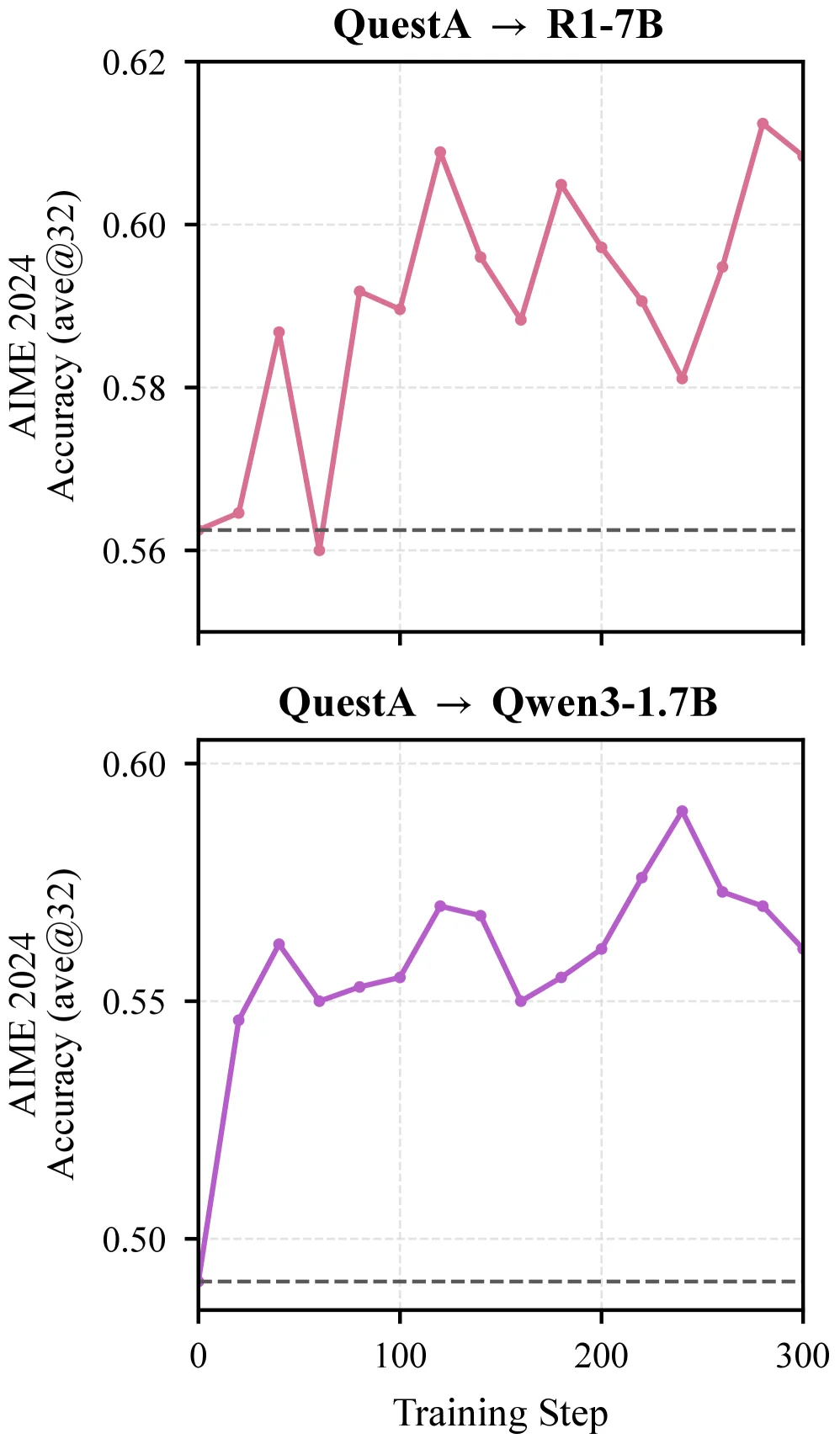
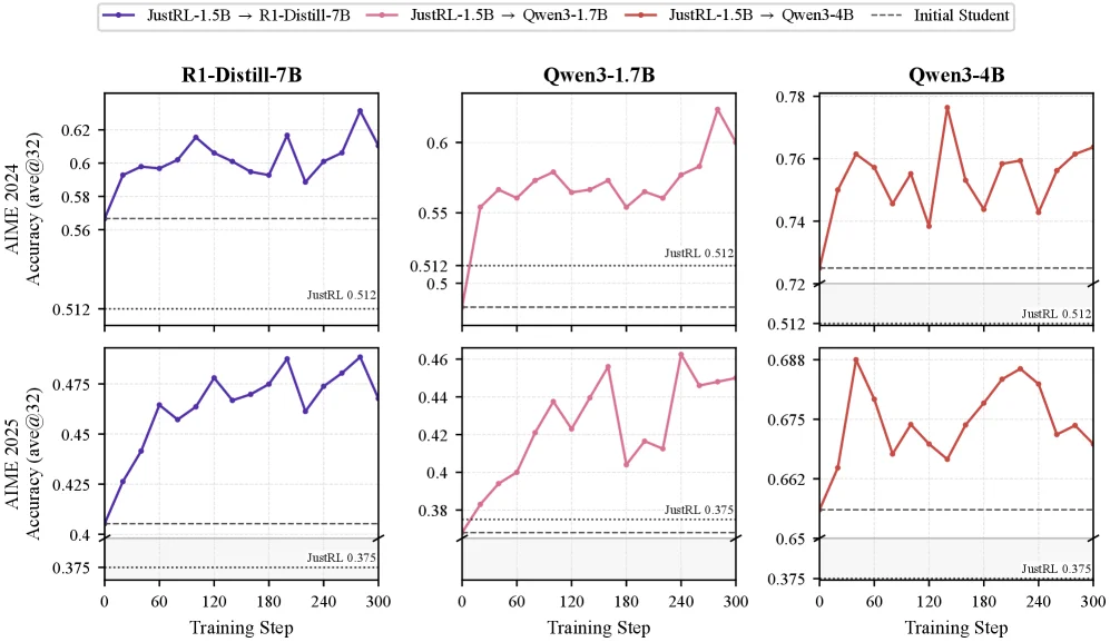
Figure 2 : Direct-OPD transfers RL-induced policy shifts across teacher pairs and student families. Left: R1-Distill-1.5B → \rightarrow JustRL-1.5B transfer into R1-Distill-7B, Qwen3-1.7B, and Qwen3-4B, evaluated on AIME 2024 and AIME 2025. Right: Nemotron-1.5B → \rightarrow QuestA-Nemotron-1.5B transfer into R1-Distill-7B and Qwen3-1.7B on AIME 2024. The two teacher pairs come from different training data and pipelines, showing that Direct-OPD is not specific to a single post-RL teacher.

This figure (Figure 2) from the paper Weak-to-Strong Generalization via Direct On-Policy Distillation illustrates how Direct-OPD (Direct On-Policy Distillation) transfers "policy shifts induced by reinforcement learning (RL) in weak models" to "stronger target models" to improve their reasoning ability (measured by accuracy on AIME benchmarks). We break down the figure:

1. Structure and Components of the Figure

The figure is organized into two rows (corresponding to two AIME benchmarks: AIME 2024 and AIME 2025) and three columns (corresponding to three "target student models": R1-Distill-7B, Qwen3-1.7B, Qwen3-4B). Each subplot shows the result of a "teacher-student" transfer:

  • X-axis (Training Step): Number of training steps (from 0 to 300), representing the Direct-OPD training process on the target student model.
  • Y-axis (Accuracy (ave@32)): Average accuracy of the model on the AIME test set ("@32" may refer to testing sampling/evaluation settings).
  • Curves and Legend:
  • Different colored curves correspond to different "teacher-student" transfer pairs (e.g., blue: JustRL-1.5B → R1-Distill-7B; pink: JustRL-1.5B → Qwen3-1.7B; red: JustRL-1.5B → Qwen3-4B).
  • Dashed line ("Initial Student"): The initial accuracy of the target student model before Direct-OPD training (the "JustRL" baseline, e.g., "JustRL 0.512" or "JustRL 0.375" in the legend, indicating initial performance).
  • Subplot Groups:
  • Upper part (AIME 2024): Shows the effect of distilling the policy shift from a "weak teacher" (JustRL-1.5B, trained with JustRL) to three stronger target models (R1-Distill-7B, Qwen3-1.7B, Qwen3-4B).
  • Lower part (AIME 2025): Similar to the upper part but evaluates another AIME benchmark (AIME 2025) to verify method generalization.

2. How Direct-OPD Works (Understood from the Figure)

The core of Direct-OPD is to "transfer the RL policy shift of the weak model", rather than directly transferring the weak model's final policy. Specifically:

  • Step 1: Train the "Weak Teacher": Select a smaller model (e.g., JustRL-1.5B) and train it with RL (here, JustRL) to obtain a "policy shift" (i.e., RL makes it more likely to take certain actions/decisions than the initial model).
  • Step 2: Extract Policy Shift: Compare the post-RL state (model after RL training) and the pre-RL state (initial JustRL model) of the "weak teacher", and calculate their "log-ratio" — this ratio reflects "which actions RL made the weak model more/less likely to take".
  • Step 3: Distill to Strong Student: Use this "policy shift signal" (log-ratio) as an implicit reward and apply it to the own On-Policy states of the stronger target student model (e.g., R1-Distill-7B, Qwen3-1.7B, Qwen3-4B) during training. Thus, the strong model does not need to perform expensive RL training itself but directly reuses the RL supervision signal from the weak model.

From the curve changes in the figure, we can see: The accuracy of all transferred models is significantly higher than the "Initial Student" dashed line, indicating that Direct-OPD successfully transfers the RL gains of the weak model to the strong model. For example: - For R1-Distill-7B (upper-left subplot), the blue curve (JustRL-1.5B→R1-Distill-7B) rises from ~0.56 to ~0.62 or above, far higher than the dashed line (~0.512). - For Qwen3-1.7B (upper-middle subplot), the pink curve rises from ~0.512 to ~0.6 or above, also far higher than the dashed line. - For Qwen3-4B (upper-right subplot), the red curve rises from ~0.72 to ~0.76 or above, significantly higher than the dashed line.

3. Results and Conclusions (What Can We Conclude from the Figure?)

  • Performance Improvement: The accuracy of all target models (R1-Distill-7B, Qwen3-1.7B, Qwen3-4B) on AIME 2024 and AIME 2025 is significantly improved by Direct-OPD, and the improvement is much larger than the initial student's performance.
  • Generalization: Different teacher pairs (e.g., JustRL-1.5B→R1-Distill-7B, JustRL-1.5B→Qwen3-1.7B, etc.) and different student model families (R1-Distill, Qwen3) benefit, indicating that Direct-OPD does not depend on specific teachers or student models.
  • Efficiency: Although the figure does not directly show time, the paper abstract mentions "improving Qwen3-1.7B from 48.3% to 58.3% in just 4 hours (8 A100 GPUs)", and combined with the training steps (0-300) in the figure, it shows that Direct-OPD has high training efficiency, avoiding repeated expensive RL training on strong models.

In summary, this figure intuitively shows the core idea of Direct-OPD — "transferring the RL policy shift of the weak model, rather than directly transferring the policy" — and proves through accuracy curves that the method can effectively improve the reasoning ability of strong models and has generalization across teachers and student models.

Figure 2 : Direct-OPD transfers RL-induced policy shifts across teacher pairs and student families. Left: R1-Distill-1.5B → \rightarrow JustRL-1.5B transfer into R1-Distill-7B, Qwen3-1.7B, and Qwen3-4B, evaluated on AIME 2024 and AIME 2025. Right: Nemotron-1.5B → \rightarrow QuestA-Nemotron-1.5B transfer into R1-Distill-7B and Qwen3-1.7B on AIME 2024. The two teacher pairs come from different training data and pipelines, showing that Direct-OPD is not specific to a single post-RL teacher.

This figure (corresponding to "Left" in Figure 2 of the paper) demonstrates how Direct - OPD transfers the RL - induced policy shift from a weak teacher model to a strong student model to improve the student's reasoning accuracy on the AIME 2024 task.

Components of the Figure and Information Flow

  • Two Sub - plots: They correspond to different "teacher - student" transfer pairs.
  • Top Sub - plot (QuestA → R1 - 7B): The horizontal axis is "Training Step" (ranging from 0 to 300), and the vertical axis is "AIME 2024 Accuracy (ave@32)" (ranging from 0.56 to 0.62). The pink line shows the change in the accuracy of the student model (R1 - 7B) during training after applying the policy shift from QuestA (a weak teacher trained with RL) to it. The dashed line (around 0.56) may be a baseline (such as the initial accuracy of the student model or the accuracy of the weak teacher).
  • Bottom Sub - plot (QuestA → Qwen3 - 1.7B): Both the horizontal axis (training step, 0 to 300) and the vertical axis (AIME 2024 accuracy, ave@32) have the same meaning as the top sub - plot. The purple line shows the accuracy change of the student model (Qwen3 - 1.7B) during training after the policy shift transfer.
  • Data Flow Logic: A weak teacher model (e.g., QuestA) is trained with RL first. The "policy shift" of its strategy (i.e., the change in the probability of certain actions) is extracted by Direct - OPD (by comparing the log - ratio of the teacher's pre - training and post - training states as an implicit reward). Then, this reward signal is applied to the on - policy states of a strong student model (e.g., R1 - 7B, Qwen3 - 1.7B) so that the student model can learn this policy shift and improve its accuracy. The figure visualizes the effect of this transfer process through the change of accuracy with the increase of training steps: as the training steps increase, the accuracy of the student model generally rises (although there are fluctuations), indicating that the policy shift effectively improves the student's reasoning ability.

How the Method Works (Understood from the Figure)

  • Selection of Weak Teacher: QuestA is used as the weak teacher in the figure (trained with RL, such as the RLVR method). The advantage of the weak teacher is that the cost of generating rollouts is low, so it is suitable for RL training first.
  • Extraction of Policy Shift: By comparing the "pre - training" and "post - training (after RL)" states of the weak teacher, the signal of the policy shift (log - ratio) is obtained. This signal reflects which actions RL training makes the weak model more or less likely to take.
  • Application to Strong Student: This policy shift signal is used as an implicit reward and applied to the on - policy training of the strong student model (e.g., R1 - 7B, Qwen3 - 1.7B). During its own training process, the student model adjusts its strategy according to this signal, thus improving its accuracy on the AIME 2024 task.
  • Visualization of the Training Process: The line chart in the figure shows the change of the student model's accuracy at different training steps. For example, in the top sub - plot, the accuracy of R1 - 7B starts from about 0.56 and generally rises to about 0.61 or above as the training steps increase, with fluctuations in between but an overall upward trend; in the bottom sub - plot, the accuracy of Qwen3 - 1.7B starts from about 0.50 and rises to about 0.59 or above, also with fluctuations but an overall upward trend.

Results and Conclusions (Understood from the Figure)

  • Coordinates and Comparison: The horizontal axis is the training step (0 to 300), and the vertical axis is the accuracy of AIME 2024 (ave@32). The dashed line in each sub - plot is a baseline (possibly the initial accuracy of the student model or the accuracy of the weak teacher).
  • Conclusions:
  • For the "QuestA → R1 - 7B" transfer, the accuracy of the student model (R1 - 7B) is significantly improved during training, from about 0.56 to about 0.61 or above, indicating that the Direct - OPD method can effectively transfer the RL policy shift of the weak teacher to the strong student model and improve its reasoning ability.
  • For the "QuestA → Qwen3 - 1.7B" transfer, the accuracy of the student model (Qwen3 - 1.7B) is increased from about 0.50 to about 0.59 or above, which also verifies the effectiveness of the method.
  • Overall, the Direct - OPD method can improve the accuracy of different strong student models on the AIME 2024 task by transferring the RL - induced policy of the weak model, indicating that the method is not dependent on a specific weak teacher or strong student model and has generality (which also conforms to the statement in the caption that it is "not specific to a single post - RL teacher").

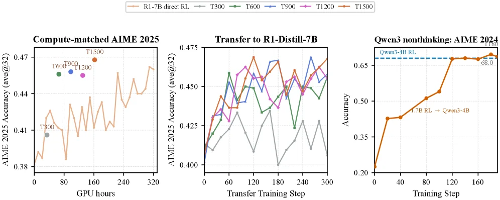
Figure 3 : Running RL on a small model and transferring its policy shift with Direct-OPD beats running RL directly on the large target, at equal compute. We compare two routes to improving R1-Distill-7B: direct RL on R1-Distill-7B, versus a weak-to-strong route that runs RL on the smaller R1-Distill-1.5B and transfers the resulting policy shift into R1-Distill-7B with Direct-OPD. T N N denotes the transfer that uses the R1-Distill-1.5B RL checkpoint at step N N as the post-RL teacher π T \pi_{T} , with the base model as π T ref \pi_{T_{\mathrm{ref}}} . Left: AIME 2025 accuracy against total GPU-hours; the wiggly curve is direct R1-Distill-7B RL, and each T N N point sums its small-model RL cost and the short Direct-OPD transfer. Later transfers (T600–T1500) sit above the direct-RL curve at equal compute—higher accuracy for less compute. Middle: Direct-OPD transfer trajectories into R1-Distill-7B from the five small-teacher checkpoints; the early T300 carries a weaker shift than T900–T1500. Right: the same recipe with Qwen3 non-thinking models—transferring a Qwen3-1.7B RL shift into Qwen3-4B reaches the 68.0 68.0 accuracy of direct Qwen3-4B RL (dashed) on AIME 2024.

This figure contains three subplots, which sequentially demonstrate from left to right the performance comparison between weak-to-strong transfer (Direct - OPD) and direct reinforcement learning (direct RL) in different scenarios, the transfer training process, and the results of specific model transfers, with the core being to verify that the method of "doing RL on a small model and then transferring it to a large model" is better than "doing RL directly on a large model".

Left Subplot: Compute - matched AIME 2025 (Accuracy of AIME 2025 with Matched Computation)

  • Axes: The horizontal axis is GPU hours (total GPU time, measuring computational cost), and the vertical axis is AIME 2025 Accuracy (avg@32) (the average accuracy of AIME 2025, where @32 may refer to the number of samples or settings during inference).
  • Meaning of Curves/Points:
  • Orange "wiggly curve": Represents the change in accuracy of doing RL directly on a large model (R1 - Distill - 7B) over GPU time. The curve fluctuates but generally shows an upward trend over time.
  • Colored points (T300, T600, T900, T1200, T1500): Represent the results of weak - to - strong transfer (Direct - OPD). Here, "T N" means using the RL checkpoint of a small model (R1 - Distill - 1.5B) at training step N as the "post - RL teacher π_T", and combining it with the "pre - RL reference π_T_ref" of the small model for Direct - OPD transfer. For example, T300 is the transfer at step 300, and T1500 is the transfer at step 1500. The "computational cost" of each point is the RL cost of the small model plus the short - time cost of Direct - OPD transfer.
  • Conclusion: Under equal computational cost, the accuracy of later transfers (such as T600 - T1500) is higher than the curve of direct RL ("Later transfers...higher accuracy for less compute"). This shows that doing RL on a small model and then transferring it to a large model can achieve better performance with the same computational resources.

Middle Subplot: Transfer to R1 - Distill - 7B (Training Trajectory of Transferring to R1 - Distill - 7B)

  • Axes: The horizontal axis is Transfer Training Step (transfer training step), and the vertical axis is AIME 2025 Accuracy (avg@32).
  • Meaning of Curves: Different colored curves correspond to different small - model RL checkpoints (T300, T600, T900, T1200, T1500) as teachers, and the change in accuracy during the process of transferring the strategy (through Direct - OPD) to R1 - Distill - 7B. For example, the orange curve corresponds to the teacher at T1500, and the green one corresponds to T600, etc.
  • Conclusion: The "strategy transfer strength" of early transfers (such as T300) is weaker than that of later transfers (such as T900 - T1500), because the teacher of later transfers (the small model after more training steps) has a more effective RL - induced strategy transfer. From the curve trend, as the transfer training step increases, the accuracy gradually improves, and the transfer effect of later teachers is better.

Right Subplot: Qwen3 nonthinking: AIME 2024 (Accuracy of Qwen3 Non - thinking Model on AIME 2024)

  • Axes: The horizontal axis is Training Step (training step), and the vertical axis is Accuracy (accuracy).
  • Meaning of Curves/Lines:
  • Orange curve: Represents the change in accuracy of transferring the RL strategy of Qwen3 - 1.7B (through Direct - OPD) to Qwen3 - 4B over the training step. The curve rises rapidly from a low accuracy and finally reaches 68.0.
  • Blue dashed line: Represents the accuracy of doing RL directly on Qwen3 - 4B ("Qwen3 - 4B RL (dashed)"), and its accuracy is also around 68.0.
  • Conclusion: By transferring the RL strategy of Qwen3 - 1.7B to Qwen3 - 4B through Direct - OPD, when the training step is sufficient, it can achieve the same accuracy as doing RL directly on Qwen3 - 4B ("reaches the 68.0 accuracy of direct Qwen3 - 4B RL"). This verifies the effectiveness of the method in the Qwen3 model series.

Operational Logic of the Method (Inferred from the Figures):

  1. Weak - model RL Stage: Run reinforcement learning (RL) on a small model (such as R1 - Distill - 1.5B, Qwen3 - 1.7B) to obtain "post - RL teacher" checkpoints at different training steps (these checkpoints contain the strategy transfer brought by RL, but the limitations of the small model lead to limitations in the strategy).
  2. Strategy Transfer (Direct - OPD) Stage: Compare the "post - RL teacher" with the "pre - RL reference" of the small model, calculate their log - ratio (as an implicit dense reward), and then apply this reward signal to the "on - policy state" of the stronger target model (such as R1 - Distill - 7B, Qwen3 - 4B) (that is, the state generated by the target model under its own strategy). In this way, the target model does not need to run RL with sparse rewards by itself, but directly reuses the RL supervision signal of the weak model.
  3. Effect Verification: By comparing the accuracy of "doing RL directly on a large model" and "weak - model RL + Direct - OPD transfer" (left figure), the change in accuracy during the transfer training process (middle figure), and the results of specific model transfers (right figure), it is proved that this method can make the strong model achieve better performance with equal or less computational cost, and even achieve the effect of doing RL directly on a large model.

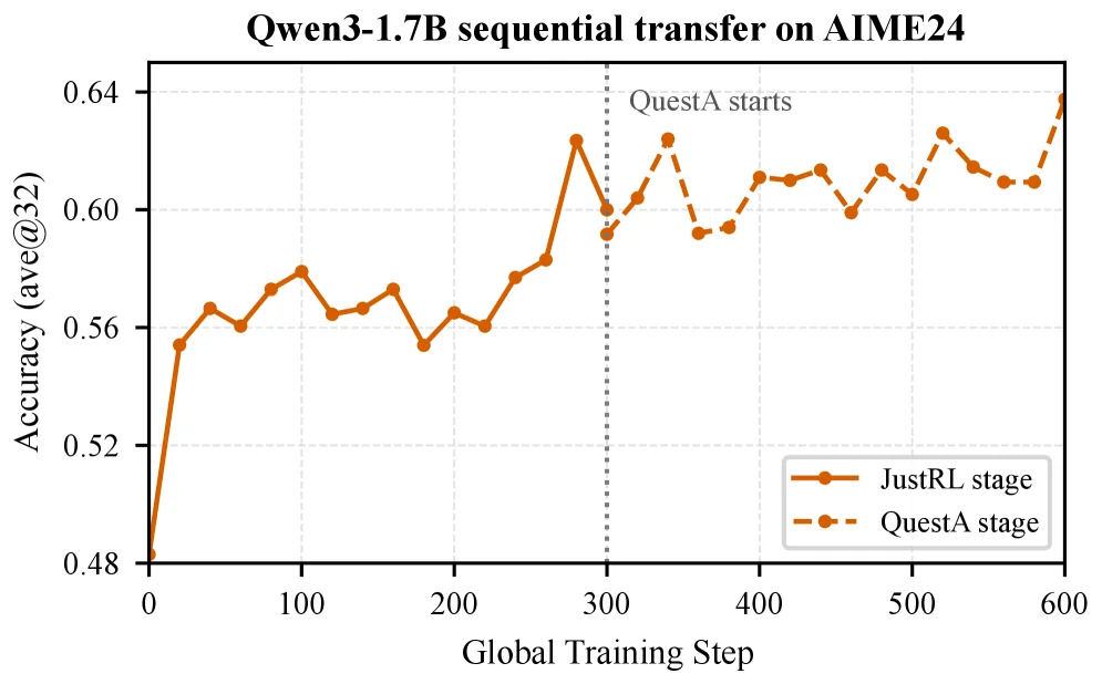
Figure 4 : Sequential policy-shift transfer into Qwen3-1.7B on AIME 2024. Left: the AIME 2024 trajectory after aligning the second stage to global steps 300–600. Right: endpoint scores on AIME 2024/2025. The first stage uses the R1-Distill-1.5B → \rightarrow JustRL-1.5B signal; the second stage continues from that checkpoint with the Nemotron-1.5B → \rightarrow QuestA-Nemotron-1.5B signal.

This diagram illustrates the process of enhancing the Qwen3-1.7B model's capabilities through sequential policy-shift transfer on the AIME2024 benchmark. The core focus is explaining how "weak-to-strong generalization" methods (e.g., Direct-OPD from the paper) reuse weak model reinforcement learning (RL) supervision signals in stages.

Diagram Components and Information Flow:

  • X-axis (Global Training Step): Represents global training steps (0–600), showing the training progress. The process has two main phases: JustRL stage (solid orange line) and QuestA stage (dashed orange line), separated by a vertical dashed line ("QuestA starts") at step 300.
  • Y-axis (Accuracy (ave@32)): Measures the model’s accuracy (average over 32 samples) on AIME2024, ranging from 0.48 to 0.64, evaluating reasoning performance.
  • Two Curves:
  • JustRL stage (solid line with dots): Corresponds to the first training phase, using signals from "R1-Distill-1.5B → JustRL-1.5B" (from the caption’s context). This phase involves a weak model (e.g., R1-Distill with 1.5B parameters) improving its strategy via RL, with accuracy gradually rising (from ~0.48 to ~0.62, peaking at step 300).
  • QuestA stage (dashed line with dots): Corresponds to the second phase, starting at step 300. It reuses the first phase’s RL supervision signals (i.e., log-ratio of weak model vs. pre-RL version as implicit rewards) for a stronger target model (Qwen3-1.7B). Accuracy continues to fluctuate upward after step 300, approaching ~0.64 at step 600, demonstrating the effectiveness of sequential transfer.

Methodology Logic (From the Diagram):

  1. First Phase (JustRL): Train a weak model (e.g., low-parameter model) via RL, enabling it to learn "policy transfer" (which actions/decisions improve performance) through interaction with the environment (AIME2024’s reasoning task). The output is the weak model’s post-RL state and a comparison with its pre-RL state (log-ratio, representing RL-driven strategy changes).
  2. Second Phase (QuestA/Sequential Transfer): Use the "policy transfer signal" (log-ratio) from the first phase as an implicit reward for the stronger target model’s (Qwen3-1.7B) on-policy state. Instead of re-running sparse-reward RL on the strong model (costly), it directly reuses the weak model’s RL supervision to guide strategy updates. The dashed line’s upward trend after step 300 confirms this "sequential transfer" effectively boosts the strong model’s performance.

Results and Conclusions (From the Diagram):

  • Axes and Comparison: The x-axis shows training steps (0–600), and the y-axis shows accuracy. JustRL stage (solid line) gradually improves accuracy from steps 0–300, while QuestA stage (dashed line) continues improving afterward, with final accuracy significantly higher than the initial ~0.48.
  • Conclusion: Sequential policy transfer (e.g., Direct-OPD) can reuse weak model RL supervision signals to effectively enhance a strong model’s reasoning ability without retraining it. The diagram shows Qwen3-1.7B’s AIME2024 accuracy rises from ~0.48 to ~0.64 (by step 600), validating the method. Additionally, this approach supports sequential combination of multiple policy transfers (implied by multi-stage transfers in the diagram), further amplifying performance.

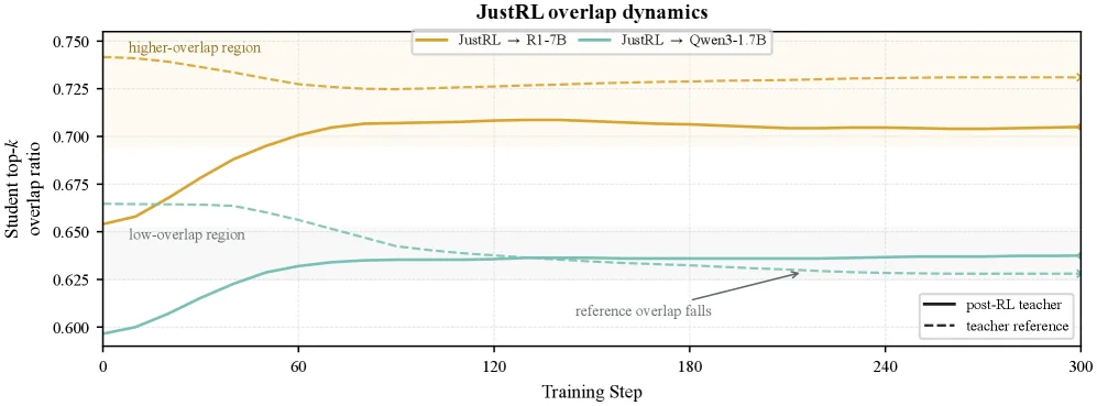
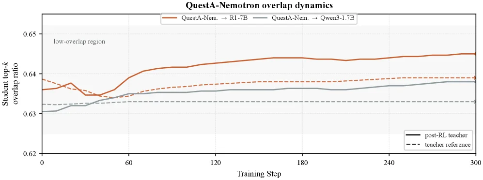
Figure 5 : Teacher–student top- k k overlap during Direct-OPD training. Left: R1-Distill-1.5B → \rightarrow JustRL-1.5B teacher pair. Right: Nemotron-1.5B → \rightarrow QuestA-Nemotron-1.5B teacher pair. Solid curves measure overlap with the post-RL teacher, and dashed curves measure overlap with the teacher reference. The pattern-aligned R1-Distill transfer enters a higher-overlap regime, while the cross-pattern transfers remain lower and do not become imitation of the post-RL teacher.

This figure is from the paper "Weak - to - Strong Generalization via Direct On - Policy Distillation" and shows the overlap dynamics of teacher - student top - k during Direct - OPD training (specifically for JustRL - related cases). First, let's look at the axes: the horizontal axis is "Training Step" (ranging from 0 to 300), representing the progress of training; the vertical axis is "Student top - k overlap ratio" (ranging from 0.600 to 0.750), measuring the overlap between the student model's top - k actions and those of the teacher - related models.

Now, let's analyze the curves and legends: - The solid orange curve represents the case of "JustRL → R1 - 7B", and the dashed cyan curve represents "JustRL → Qwen3 - 1.7B". Additionally, there are two reference lines: the black solid line is "post - RL teacher" (the teacher model after reinforcement learning), and the black dashed line is "teacher reference" (a reference model of the teacher). - There are two region labels: "higher - overlap region" (corresponding to the area near the initial part of the orange curve) and "low - overlap region" (corresponding to the area near the initial part of the cyan curve). There is also an arrow labeled "reference overlap falls" (pointing to the trend of the cyan dashed line).

To understand how the method works: The core of Direct - OPD is to transfer the strategy shift induced by reinforcement learning (RL) from a weak teacher model, rather than directly distilling the final strategy of the weak teacher. From the figure, we can see that for different teacher - student pairs (here, JustRL is related to the teacher, and R1 - 7B and Qwen3 - 1.7B are students? Or vice versa? Combining the understanding of the caption, it should be the overlap rate change between the teacher - related model (such as JustRL - related) and the student models (R1 - 7B, Qwen3 - 1.7B). The solid curve (JustRL → R1 - 7B) has an overlap rate that increases from about 0.650 to above 0.700 as the training step increases, entering a relatively stable "higher - overlap region". This shows that this transfer (possibly a pattern - aligned transfer) makes the student model's overlap rate with the post - RL teacher model increase, entering a high - overlap state. The dashed curve (JustRL → Qwen3 - 1.7B) has an initial overlap rate of about 0.600, rises to about 0.630 and then stabilizes, and "reference overlap falls" (the reference overlap rate decreases). This shows that this cross - pattern transfer does not make the student model imitate the strategy of the post - RL teacher, and the overlap rate does not reach a high - overlap state.

From the perspective of results, the horizontal axis of training steps shows the change of the overlap rate between the student model and different teacher references as training progresses. The comparison objects are different teacher - student pairs (JustRL→R1 - 7B and JustRL→Qwen3 - 1.7B), as well as the overlap rates with the post - RL teacher and the teacher reference. The conclusion is that the pattern - aligned transfer (such as JustRL→R1 - 7B) will enter the high - overlap region, while the cross - pattern transfer remains at a low overlap rate and will not imitate the strategy of the post - RL teacher. This verifies the effectiveness of strategy transfer in Direct - OPD, that is, only when the teacher and student are pattern - aligned can the RL - induced strategy shift be effectively transferred to improve the overlap rate (that is, the consistency of the strategy) between the student model and the teacher model.

Figure 5 : Teacher–student top- k k overlap during Direct-OPD training. Left: R1-Distill-1.5B → \rightarrow JustRL-1.5B teacher pair. Right: Nemotron-1.5B → \rightarrow QuestA-Nemotron-1.5B teacher pair. Solid curves measure overlap with the post-RL teacher, and dashed curves measure overlap with the teacher reference. The pattern-aligned R1-Distill transfer enters a higher-overlap regime, while the cross-pattern transfers remain lower and do not become imitation of the post-RL teacher.

This diagram illustrates the dynamic changes in top-k overlap between student and teacher models during Direct-OPD (Direct Policy Distillation) training, focusing on comparing the overlap evolution of student models under two objectives: "post-RL teacher" (after reinforcement learning) and "teacher reference" (pre-RL teacher model). The goal is to validate the method's effectiveness.

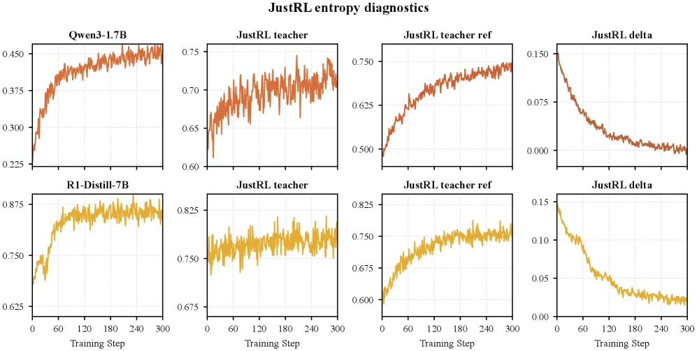
Figure 6 : Entropy diagnostics for R1-Distill-1.5B → \rightarrow JustRL-1.5B policy-shift transfer. Top row: transfer into Qwen3-1.7B. Bottom row: transfer into R1-Distill-7B. Each row shows student entropy, post-RL teacher entropy, teacher-reference entropy, and teacher entropy minus reference entropy. Actor entropy does not collapse, while the teacher/reference entropy gap narrows over training.

This figure from the paper Weak-to-Strong Generalization via Direct On-Policy Distillation visualizes entropy dynamics during reinforcement learning (RL) policy transfer, clarifying how the proposed method (Direct On-Policy Distillation) works. Here’s a detailed breakdown:

1. Chart Structure & Components

The figure has two rows (one for each target model) and four subplots per row, showing entropy trends over training steps (x-axis, 0–300):

  • Top Row: Transfer to Qwen3-1.7B (a strong target model).
  • Bottom Row: Transfer to R1-Distill-7B (another strong target model).

Each row’s subplots (left to right) represent:
- Student Entropy (e.g., Qwen3-1.7B or R1-Distill-7B): Tracks the entropy of the student (target) model’s policy.
- Post-RL Teacher Entropy (e.g., JustRL teacher): Tracks the entropy of the post-RL teacher (a weak model trained with RL).
- Teacher-Reference Entropy (e.g., JustRL teacher ref): Tracks the entropy of the teacher’s pre-RL reference model (the teacher’s policy before RL training).
- Teacher Entropy Minus Reference Entropy (e.g., JustRL delta): Tracks the gap between the post-RL teacher’s entropy and its pre-RL reference’s entropy.

2. Method Mechanism (How It Works)

The method (Direct On-Policy Distillation) aims to transfer the policy shift induced by RL on a weak teacher to a strong student, without running expensive RL on the student. Here’s how the plots illustrate this:

  • Student Entropy: The student model’s entropy (e.g., Qwen3-1.7B or R1-Distill-7B) does not collapse (entropy remains stable, not dropping to near-zero). This means the student retains policy diversity while learning from the teacher.
  • Teacher vs. Reference Entropy Gap (delta subplot): The gap between the post-RL teacher’s entropy and its pre-RL reference’s entropy narrows over training (the curve in the “delta” subplot decreases). This shows the teacher’s policy becomes more distinct from its pre-RL state (i.e., RL induces a meaningful strategy shift).
  • Entropy Transfer: The student’s entropy trends (rising then stabilizing) align with the teacher’s entropy trends, implying the student learns the teacher’s RL-induced strategy shift (via the “dense implicit reward” mechanism described in the paper).

3. Results & Conclusions

From the plots:
- Entropy Stability: Student models (e.g., Qwen3-1.7B, R1-Distill-7B) do not experience entropy collapse (their entropy remains stable, not too low or too high).
- Strategy Shift Transfer: The “delta” subplot (teacher entropy − reference entropy) shows the gap narrows over training, confirming the teacher’s RL-induced strategy shift is transferred to the student.
- Generalizability: The method works across different target models (Qwen3-1.7B and R1-Distill-7B), as shown by consistent entropy trends.

In short, the figure demonstrates that Direct On-Policy Distillation successfully transfers the weak teacher’s RL-supervised strategy shift to the strong student, while preserving the student’s policy diversity (no entropy collapse) and reducing the gap between the teacher’s post-RL and pre-RL policies.

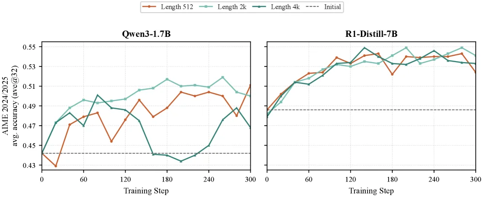
Figure 7 : Response-length sweep for R1-Distill-1.5B → \rightarrow JustRL-1.5B transfer with fixed KL coefficient 1 1 . We report the average of AIME 2024 and AIME 2025 validation accuracy (ave@32) during training for Qwen3-1.7B and R1-Distill-7B students. The 2k setting gives stable validation behavior across the two students, while shorter or longer rollouts do not consistently improve the validation curves.

This figure is from the paper "Weak-to-Strong Generalization via Direct On-Policy Distillation" and illustrates the process and effectiveness of transferring knowledge from a "weak" teacher model, trained via reinforcement learning (RL), to a "strong" student model under different response lengths (rollout lengths). Specifically, it shows the Qwen3-1.7B → JustRL-1.5B transfer (with a fixed KL coefficient of 1) and evaluates the performance on two student models: Qwen3-1.7B and R1-Distill-7B.

Let's break down the components of the figure:

  1. Overall Layout: The figure contains two subplots, each corresponding to a different student model:

    • The left subplot is titled "Qwen3-1.7B," indicating the student model is Qwen3-1.7B.
    • The right subplot is titled "R1-Distill-7B," indicating the student model is R1-Distill-7B. Each subplot shows the performance of the student model during training under different response length settings.
  2. X-axis (Horizontal Axis): The x-axis for both subplots is labeled "Training Step," ranging from 0 to 300. This represents the progress of the training process.

  3. Y-axis (Vertical Axis): The y-axis for both subplots is labeled "AIME 2024/2025 ave. accuracy (ave@32)," which is a metric measuring the model's reasoning ability. Higher values indicate better performance. "ave@32" likely refers to the average accuracy over 32 samples or steps.

  4. Curves and Legend:

    • Each subplot contains four curves, differentiated by color and style, representing different "response-length" settings:
      • Orange solid line (Length 512): Represents the setting with a response length of 512 tokens.
      • Cyan dashed line (Length 2k): Represents the setting with a response length of 2000 tokens.
      • Dark green solid line (Length 4k): Represents the setting with a response length of 4000 tokens.
      • Black dashed line (Initial): Represents the initial performance of the student model (i.e., its accuracy before distillation begins).
    • These curves show how the accuracy of the student model changes during training for each response length setting.
  5. Data Flow and Information Interpretation:

    • The core of the experiment is "distillation": transferring knowledge learned by a smaller, RL-trained "weak" teacher model (R1-Distill-1.5B) to a larger student model (Qwen3-1.7B or R1-Distill-7B).
    • "Response-length sweep" means the experimenters tested different response length settings to find the optimal one.
    • For each student model and each response length setting, the accuracy during training was recorded and plotted as a curve.
    • We can observe the trend of each curve:
      • In the Qwen3-1.7B subplot, the curve for Length 2k (cyan dashed line) performs the best in the later stages of training (around step 200 onwards), achieving the highest accuracy. The curves for Length 512 (orange solid line) and Length 4k (dark green solid line) are more volatile or perform worse at certain points.
      • In the R1-Distill-7B subplot, all three curves for different lengths (512, 2k, 4k) show an upward trend during training and stabilize in the later stages (around step 100 onwards) with high accuracy. The curves for Length 2k (cyan dashed line) and Length 4k (dark green solid line) appear to perform the best, while the curve for Length 512 (orange solid line) closely follows.
    • The black dashed line (Initial) represents the initial accuracy of the student model. All colored curves start from this initial point and gradually rise during training, indicating that the distillation process indeed improves the model's performance.
  6. Method Operation Revealed:

    • This figure demonstrates the practical application of the "Direct On-Policy Distillation (Direct-OPD)" method. The core idea is to leverage the knowledge from a "weak" teacher model that has already been improved by RL on a smaller model, rather than running sparse-reward RL directly on the target model.
    • Specifically, Direct-OPD compares the RL-trained teacher model with its own pre-RL reference model and treats their log-ratio as a dense implicit reward for the student model.
    • In this figure, we see that by performing RL training on a smaller teacher model and then distilling the learned knowledge to a larger student model, the student model's performance is significantly improved.
    • The "response-length sweep" is to find an optimal response length setting for the most effective distillation. The results show that for these two student models, a response length of 2k provides the most stable and best validation behavior.
  7. Comparison Objects and Conclusion:

    • Comparison Objects:
      • Different student models: Qwen3-1.7B and R1-Distill-7B.
      • Different response length settings: 512, 2k, and 4k.
      • The initial performance of the student model (Initial) versus its performance during training.
    • Conclusion:
      • As stated in the original caption: "The 2k setting gives stable validation behavior across the two students, while shorter or longer rollouts do not consistently improve the validation curves." (2k 设置在两个学生模型上都提供了稳定的验证行为,而更短或更长的 rollout 并没有持续改善验证曲线。)
      • This means that in this experiment, choosing a response length of 2000 tokens is optimal because it provides the most stable and best performance improvement.
      • The curves in the figure clearly show this: on both student models, the curve for Length 2k performs the best or comparably to other lengths, while curves for other lengths are unstable or worse.
      • Overall, this figure proves the effectiveness of the Direct-OPD method, i.e., the reasoning ability of a larger student model can be improved by distilling knowledge from a smaller, RL-trained teacher model. And choosing an appropriate response length is crucial for achieving optimal performance.

In summary, this figure intuitively explains how the Direct-OPD method works and why choosing a specific response length (e.g., 2k) is important for optimizing performance by showing how the student model's accuracy changes during training under different response length settings. It clearly demonstrates how the distillation process improves the student model's performance and points out the importance of selecting the right response length setting.

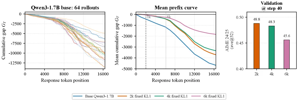
Figure 8 : Short-horizon Direct-OPD training changes behavior beyond the supervised prefix. On a fixed set of 64 long rollouts we track the cumulative gap G T = ∑ t ≤ T g t G_{T}=\sum_{t\leq T}g_{t} , where g t g_{t} weights, over the actor’s top-16 tokens at position t t , the log-probability the post-RL teacher (JustRL) assigns minus that of the reference (R1-Distill-1.5B); higher G T G_{T} means the actor’s likely tokens look more like the post-RL teacher, while lower means the actor remains closer to the reference. Left: the 64 per-rollout trajectories for the untrained Qwen3-1.7B actor all drift negative—its long rollouts are reference-like, and this is not driven by a single outlier. Middle: the mean G T G_{T} for the base actor and for actors trained with 2k/4k/6k response length (40 steps, fixed KL = 1 {=}1 ); every trained actor sits above the base across the full ∼ \sim 16k positions, and the 2k actor shifts well past its 2k training horizon (dashed line). Right: AIME 2024/2025 (ave@32) at the same 40-step checkpoint—the 2k setting validates best.

This figure from the paper Weak-to-Strong Generalization via Direct On-Policy Distillation illustrates the behavioral changes induced by the Direct-OPD (Direct On-Policy Distillation) method, with three subplots analyzed sequentially from left to right:

Left Subplot: "Qwen3-1.7B base: 64 rollouts"

  • X-axis: Response token position (ranging from 0 to 16,000), representing the length position of the generated sequence.
  • Y-axis: Cumulative gap \( G_T \) (calculated as \( G_T=\sum_{t \leq T} g_t \)), where \( g_t \) weights the log-probability difference between the post-RL teacher (JustRL) and the reference model (R1-Distill-1.5B) over the actor’s top-16 tokens at position \( t \). A higher \( G_T \) means the actor’s (untrained Qwen3-1.7B here) token distribution is more similar to the post-RL teacher; a lower \( G_T \) means it stays closer to the reference.
  • Content: Multiple colored curves represent the trajectories of 64 long rollouts. All untrained Qwen3-1.7B actors’ trajectories drift negative—indicating their long rollouts are more reference-like, and this trend is not driven by a single outlier. This shows the baseline state: Without Direct-OPD training, the model’s behavior (token distribution) is closer to the reference model than to the post-RL teacher.

Middle Subplot: "Mean prefix curve"

  • X-axis: Response token position (0 to 16,000), representing the sequence position.
  • Y-axis: Mean cumulative gap \( G_T \) (average \( G_T \) across models: base, 2k, 4k, 6k settings), calculated similarly to the left subplot.
  • Curves & Comparisons:
  • Blue curve: Base Qwen3-1.7B (untrained baseline), with the lowest \( G_T \) (most negative), meaning its behavior is most reference-like.
  • Orange (2k fixed KL1), green (4k fixed KL1), pink (6k fixed KL1) curves: Models trained with 2k, 4k, 6k response lengths (40 steps, fixed KL=1). All trained models have higher \( G_T \) than the baseline (blue) across ~16k positions. Notably, the 2k-trained model (orange) continues to increase \( G_T \) (shift positive) beyond its 2k training horizon (dashed line, ~2000), meaning the training effect persists after the training sequence length.
  • Method Implication: This shows Direct-OPD’s effectiveness: By using the log-ratio of the post-RL teacher and reference as an implicit reward, training a stronger student (Qwen3-1.7B) makes its behavior more like the post-RL teacher, and this effect lasts beyond the training horizon.

Right Subplot: "Validation @ step 40"

  • X-axis: Training settings (2k, 4k, 6k, corresponding to the middle subplot’s settings).
  • Y-axis: AIME 2024/2025 (ave@32) (average score on AIME 2024/2025, with “@32” likely a evaluation setup like averaging 32 samples).
  • Data & Conclusion:
  • 2k (orange): Score = 48.8;
  • 4k (green): Score = 48.3;
  • 6k (pink): Score = 45.6.
  • Conclusion: At the same 40-step checkpoint, the 2k setting has the highest validation score, meaning 2k response length performs best in Direct-OPD training.

Overall Logic & Method Explanation

The figure explains Direct-OPD’s workflow and results through three subplots (baseline behavior → trained behavior → validation performance):

  1. Problem Context: RL with verifiable rewards (RLVR) improves language-model reasoning but is costly for new strong models (requires many rollouts during training). Direct-OPD aims to reuse weak models’ RL supervision to improve strong models without sparse-reward RL on the target.

  2. Method Core: Direct-OPD compares a post-RL weak teacher and its pre-RL reference, treating their log-ratio as an implicit reward for the strong student’s on-policy states. This reuses the weak model’s RL-induced policy shift (without sparse-reward RL on the target).

  3. Figure Validation:

  4. Left: Untrained strong model (Qwen3-1.7B) behaves like the reference (initial state: behavior differs from the post-RL teacher).
  5. Middle: Trained models (via Direct-OPD) have higher \( G_T \) (more like the post-RL teacher), and effects persist beyond the training horizon (e.g., 2k-trained model improves after 2k tokens).
  6. Right: 2k setting has the highest validation score, showing effective performance improvement.

In short, the figure uses “cumulative gap \( G_T \)” and “validation performance” to show how Direct-OPD reuses weak models’ RL signals to change strong models’ behavior and improve validation performance.

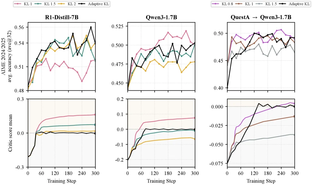
Figure 9 : The best KL coefficient is pair-dependent, and adaptive KL pulls the mean teacher-shift reward toward a balanced regime. 2k-response runs across fixed KL coefficients, with adaptive KL as the black curve. Top row: AIME 2024/2025 validation accuracy (ave@32); bottom row: mean teacher-shift reward. The best fixed coefficient differs across teacher-student pairs, and a larger mean reward does not imply better validation. Adaptive KL instead pulls the mean reward toward zero after an initial correction, keeping the student from simply maximizing the dense teacher/reference reward.

This figure is from the paper "Weak-to-Strong Generalization via Direct On-Policy Distillation" and illustrates how model performance and rewards change when training with different KL coefficients (including adaptive KL) across various teacher-student model pairs.

Explanation of the Figure's Structure and Components

  1. Subplot Layout:
  2. The figure is divided into two rows, with three subplots in each row.
  3. The top row shows the AIME 2024/2025 validation accuracy (ave@32), while the bottom row displays the mean teacher-shift reward.
  4. Each subplot corresponds to a different teacher-student model pair:

    • Left column: R1-Distill-7B (teacher) to a student model.
    • Middle column: Qwen3-1.7B (teacher) to a student model.
    • Right column: QuestA → Qwen3-1.7B (teacher to student).
  5. Axes:

  6. The x-axis represents the training step, ranging from 0 to 300.
  7. The y-axis for the top row shows validation accuracy (avg. accuracy (ave@32)), while the y-axis for the bottom row shows the mean teacher-shift reward (Critic score mean).

  8. Curves and Colors:

  9. Each curve represents a different KL coefficient:
    • Pink: KL
    • Cyan: KL 1.5
    • Yellow: KL 2
    • Black: Adaptive KL
  10. The curve colors and styles are consistent across different model pairs for easy comparison.

How the Method Works

  1. Fixed KL Coefficients:
  2. The figure shows results using fixed KL coefficients (e.g., KL, KL 1.5, KL 2).
  3. Each fixed KL coefficient has a corresponding curve, showing validation accuracy and average reward over different training steps.

  4. Adaptive KL:

  5. The black curve represents adaptive KL, which automatically adjusts the KL coefficient during training.
  6. The goal of adaptive KL is to pull the average teacher-shift reward toward a balanced state, preventing the student model from merely maximizing dense teacher/reference rewards.

  7. Dependency of Optimal KL Coefficient:

  8. The figure indicates that the optimal fixed KL coefficient varies depending on the model pair.
  9. For example, in some model pairs, KL 1.5 may perform best, while in others, KL 2 may be superior.

  10. Relationship Between Reward and Accuracy:

  11. The figure also shows the relationship between the average teacher-shift reward and validation accuracy.
  12. A higher average reward does not necessarily mean better validation accuracy, indicating a complex relationship between the reward signal and task performance.

Conclusion

  • Advantages of Adaptive KL:
  • Adaptive KL can pull the average reward toward zero, preventing the student model from overfitting to teacher/reference rewards.
  • This method demonstrates better consistency and generalization across different model pairs.

  • Choosing the Optimal KL Coefficient:

  • The best fixed KL coefficient varies by model pair and needs to be adjusted accordingly.
  • Adaptive KL provides a more flexible and effective approach without requiring manual selection of the KL coefficient.

From this figure, we can clearly see how different KL coefficients and adaptive KL perform across various model pairs and how they affect validation accuracy and average reward. Adaptive KL generally performs better because it automatically adjusts the KL coefficient to avoid overfitting.

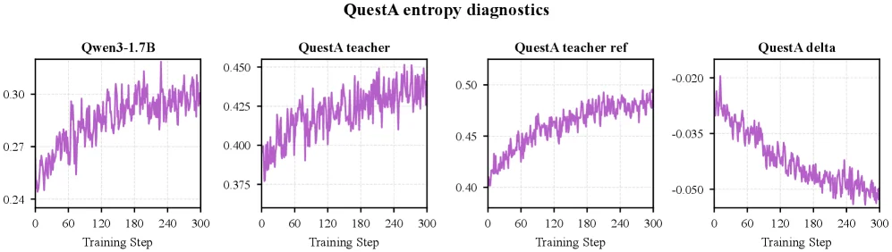
Figure 10 : Entropy diagnostics for QuestA-Nemotron into Qwen3-1.7B. The panels show student entropy, post-RL teacher entropy, teacher-reference entropy, and teacher entropy minus reference entropy. Together with Figure 6 , this shows that the non-collapse pattern is not specific to the JustRL teacher pair.

This figure (Figure 10) is from the paper "Weak-to-Strong Generalization via Direct On-Policy Distillation" and is used to display the entropy diagnosis results of "QuestA-Nemotron to Qwen3-1.7B," helping to understand the logic of strategy distribution changes in the Direct On-Policy Distillation (Direct-OPD) method. We analyze each subplot individually and then summarize the overall information:

1. Subplot Components and Information Flow

The figure contains 4 subplots, with the horizontal axis being "Training Step (训练步数)" ranging from 0 to 300, and the vertical axis representing entropy-related metrics. All curves are purple (representing the entropy trend over training steps).

  • First Subplot: Qwen3-1.7B
    Titled "Qwen3-1.7B," the vertical axis ranges approximately from 0.24 to 0.30. This curve shows the change in entropy of the student model (Qwen3-1.7B) over training steps. Entropy can be understood as the "uncertainty" or "diversity" of the strategy: higher entropy means the strategy's action distribution is more dispersed; lower entropy means the strategy is more concentrated (possibly more "certain" or "converged"). Here, we observe that entropy rises with training steps and then stabilizes, reflecting the trend of strategy changes in the student model during training.

  • Second Subplot: QuestA Teacher
    Titled "QuestA teacher," the vertical axis ranges approximately from 0.375 to 0.450. This curve shows the change in entropy of the teacher model (QuestA teacher) after reinforcement learning (RL) training over training steps. The entropy change of the teacher model reflects the impact of RL training on its strategy: from the figure, entropy increases with steps, indicating that RL training increases the strategy diversity (or uncertainty) of the teacher model (or makes it more "exploratory").

  • Third Subplot: QuestA Teacher Ref
    Titled "QuestA teacher ref," the vertical axis ranges approximately from 0.40 to 0.50. This curve shows the change in entropy of the "pre-RL reference model" of the teacher model (i.e., the original model before RL training) over training steps. The entropy change of the reference model represents the "natural strategy distribution trend of the teacher model without RL intervention," used to compare with the "post-RL teacher model" to isolate the strategy changes brought by RL.

  • Fourth Subplot: QuestA Delta
    Titled "QuestA delta," the vertical axis ranges approximately from -0.050 to -0.020. This curve shows the difference (delta = teacher entropy - reference entropy) between the teacher model's entropy (post-RL) and the reference model's entropy (pre-RL) over training steps. A positive value indicates that RL training increases the teacher model's entropy (more dispersed strategy/explorer); a negative value indicates a decrease in entropy (more concentrated strategy/exploiter). The delta in the figure gradually rises from negative (absolute value decreases), suggesting that the impact of RL training on the teacher model's entropy is "inhibiting entropy in the early stage (negative delta) and increasing entropy in the later stage (delta approaches 0 or becomes positive)"? Or more accurately, the trend of delta reflects the "RL-induced strategy transfer": what we need is the strategy change of the teacher model relative to the reference model, and this delta is the quantification of this change.

2. Visual Explanation of Method Operation (Core Logic of Direct-OPD)

The goal of Direct-OPD is to transfer the knowledge that the "weak teacher model (QuestA)" obtained through RL to the "strong target model (Qwen3-1.7B)" without directly performing sparse-reward RL on the target model (because the target model is large, and RL is costly). The core of the method is:
- First, perform RL training on the weak model (QuestA) to obtain the "post-RL teacher model";
- Then, take the "pre-RL reference model" of the weak model (the original model before training);
- Calculate the difference (delta) between the "post-RL teacher entropy" and the "pre-RL reference entropy." This difference represents the "strategy transfer signal brought by RL training to the teacher model" (i.e., which action probabilities increase/decrease due to RL);
- Use this difference as an "implicit reward" and directly apply it to the "on-policy states" of the strong target model (Qwen3-1.7B) (i.e., in the states generated by the target model under its own strategy, apply this transfer signal).

This figure visualizes this process through changes in entropy:
- Entropy of the student model (Qwen) (first figure): Shows the initial/training strategy distribution of the target model;
- Post-RL entropy of the teacher model (QuestA) (second figure): Shows the strategy distribution of the weak model after RL;
- Pre-RL entropy of the teacher model (third figure): Shows the strategy distribution of the weak model without RL;
- Difference (fourth figure): Shows the "RL-induced strategy transfer" (i.e., the difference between post-RL and pre-RL).

By comparing these four figures, we can verify that: The strategy change of the teacher model (delta) is not a "model collapse" (such as overly concentrated or random strategy) but an effective transfer brought by RL training—this is consistent with the "non-collapse pattern" conclusion in the paper: this strategy transfer pattern is not specific to a certain "JustRL teacher pair" but is reproducible (i.e., similar entropy change patterns can be observed for different teacher pairs).

3. Results and Conclusions (Information Observable from the Figure)

  • Consistency of Entropy Trends: The entropy changes in all four subplots show a trend of "rising and then stabilizing," indicating that the model's strategy gradually converges (or reaches a certain balance) during training. However, the entropy of the teacher model (post-RL) is higher than that of the reference model, and the difference (delta) reflects the contribution of RL.
  • Generality of Non-Collapse Pattern: Combined with the conclusion of "Figure 6" in the paper, this figure (Figure 10) shows that this "non-collapse pattern of strategy transfer" is not unique to a specific teacher pair (such as JustRL)—even when changing to the "QuestA-Nemotron to Qwen3-1.7B" model pair, similar entropy change patterns can be observed. This indicates that the effectiveness of the Direct-OPD method does not depend on a specific teacher model and has generality.
  • Support for Method Effectiveness: Through the difference (delta) in entropy, we can quantify the "strategy change brought by RL to the teacher model" and transfer this change as a signal to the target model. The trend of delta in the figure (from negative to positive or absolute value decreasing) indicates that RL indeed changes the strategy distribution of the teacher model, and this change can be utilized by the target model (because the entropy change of the target model also shows strategy adjustment).

Summary: This figure visualizes the core logic of the Direct-OPD method—"weak teacher model's RL training → strategy transfer (delta) → strong target model application"—through four entropy-related subplots. It proves that the "RL-induced strategy transfer" is quantifiable, transferable, and does not depend on a specific model pair, thus supporting the effectiveness of the Direct-OPD method.

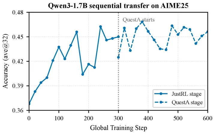
Figure 11 : Sequential policy-shift transfer into Qwen3-1.7B on AIME 2025. The QuestA-Nemotron stage is aligned after the JustRL stage using global steps 300–600, matching the AIME 2024 alignment in Figure 4 .

This figure illustrates the process of sequentially transferring a reinforcement learning (RL) policy from a smaller model (JustRL stage) to a larger target model, Qwen3-1.7B (QuestA stage), on the AIME 2025 benchmark, and its impact on accuracy.

The x-axis represents "Global Training Step," ranging from 0 to 600, indicating the timeline of the entire training process. The y-axis shows "Accuracy (ave@32)," ranging from 0.36 to 0.48, measuring the model's performance on the AIME 2025 task (average accuracy over 32 attempts).

There are two curves in the plot: 1. The solid line (blue dots) represents the "JustRL stage." This stage corresponds to the process of training a smaller teacher model using reinforcement learning to learn problem-solving strategies. From the graph, during this stage (approximately steps 0 to 300), the model's accuracy starts at around 0.36 and fluctuates upwards with increasing training steps, peaking at around 0.47. This indicates that the teacher model's performance on the task improves through RL training. 2. The dashed line (light blue dots) represents the "QuestA stage." This stage occurs after the JustRL stage and involves transferring the previously learned strategy from the teacher model to the target model, Qwen3-1.7B. According to the original figure caption, the QuestA-Nemotron stage is aligned with the JustRL stage during global steps 300-600. From the graph, after approximately step 300 (where the dashed line begins), the model's accuracy starts from a relatively high point (around 0.43) and continues to fluctuate, generally maintaining a high level, and even surpassing the peak of the pure RL stage in some points, eventually stabilizing between about 0.45 and 0.47.

A vertical dashed line labeled "QuestA starts" is positioned at around 300 global steps. This line clearly divides the two stages: the area to the left of the line is the JustRL stage, and the area to the right is the QuestA stage. This indicates that the policy transfer occurs around training step 300.

This figure reveals how the Direct On-Policy Distillation (Direct-OPD) method works: - First, RL training (the JustRL stage) is performed on a smaller model (the teacher model) to learn problem-solving strategies. The goal of this stage is to optimize the teacher model's policy through interaction with the environment (generating rollouts) and improve its accuracy on the task. - Then, when the teacher model has been trained to a certain extent (e.g., around step 300 in the figure), the learned strategy is transferred to a larger target model (Qwen3-1.7B) (the QuestA stage). This transfer process does not involve re-running RL but rather utilizes the "policy shift" learned by the teacher model during RL training. - Specifically, Direct-OPD compares the post-RL teacher model with its own pre-RL reference state and treats their log-ratio as a "dense implicit reward" for the student model (target model). This means that the information about which actions the teacher model became more or less likely to take (relative to its initial state) is used to guide the behavior of the student model in its own on-policy states. - The results in the figure clearly show that after the QuestA stage (post-transfer), the target model's accuracy not only remains at a high level but also improves in some cases. This demonstrates that the Direct-OPD method successfully leverages the RL supervision signal from the weaker teacher model to improve the stronger target model without running sparse-reward RL on the target model.

Conclusion: This figure demonstrates that through the Direct-OPD method, the strategy learned by a smaller model (teacher) via RL can be effectively transferred to a larger target model (Qwen3-1.7B), thereby improving the target model's performance without the need for expensive re-training with RL. The plot shows that after the policy transfer (QuestA stage), the model's accuracy is maintained at a high level, proving the effectiveness of the method.

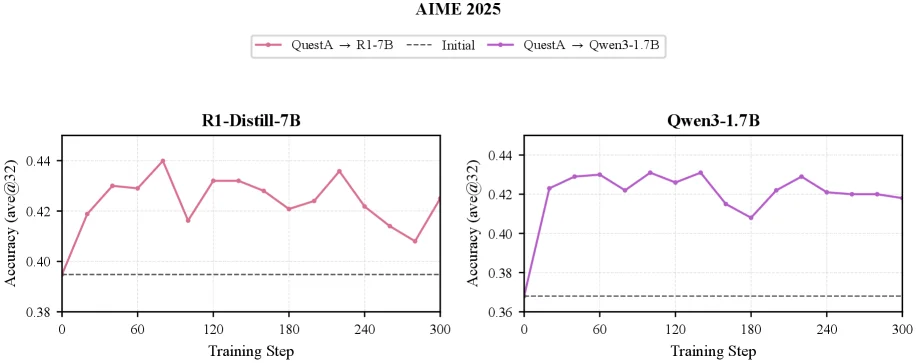
Figure 12 : QuestA transfer curves on AIME 2025 for the cross-pattern transfer setting. The main text reports the corresponding AIME 2024 curves.

This figure (Figure 12) illustrates the "QuestA transfer curve" of cross - model transfer learning in the AIME 2025 benchmark. The core is to verify how the "weak - to - strong generalization" method (such as the Direct On - Policy Distillation proposed in the paper) transfers the reinforcement learning (RL) benefits of small models to large models. The following is an analysis by modules:

1. Structure and Components of the Figure

  • Title and Scenario: The title "AIME 2025" indicates that the task is the AIME 2025 mathematical reasoning benchmark; "QuestA transfer curves" means it is the transfer learning curve of "QuestA" (a task or dataset), and "cross - pattern transfer setting" refers to the transfer across model patterns (small model → large model).
  • Sub - figures and Models: The figure contains two sub - figures, corresponding to the target model R1 - Distill - 7B (left) and Qwen3 - 1.7B (right) respectively. The horizontal axis is "Training Step (training steps)" with a range from 0 to 300; the vertical axis is "Accuracy (avg@32) (accuracy, average of 32 times)" with a range of about 0.36 to 0.44.
  • Curves and Legends:
  • Dashed line (Initial): Represents the initial accuracy of the target model (the basic performance without transfer learning).
  • Red solid line (QuestA → R1 - 7B): Indicates the change of accuracy with the increase of training steps after transferring the RL knowledge of the "QuestA" task from the small model (implied weak model) to the R1 - Distill - 7B (target model).
  • Purple solid line (QuestA → Qwen3 - 1.7B): Indicates the change of accuracy after transferring the RL knowledge of "QuestA" to the Qwen3 - 1.7B (target model).

2. Operating Logic of the Method (Inferred from the Figure)

The core method of the paper is Direct On - Policy Distillation: Instead of performing RL on the small model and then repeating it on the large model, it uses the difference between the "policy after RL training of the weak model (small model)" and "its pre - training policy" (that is, the policy shift brought by RL) as an "implicit reward" and transfers it to the "on - policy (when the policy is executed)" state of the strong model (large model). The meaning of the curves in the figure can be understood as follows: - Initial State (Dashed Line): The initial performance of the target model (for example, the Initial accuracy of R1 - Distill - 7B is about 0.39, and the Initial of Qwen3 - 1.7B is about 0.37), which is the benchmark when no knowledge is transferred. - Transfer Learning Process: The rise (or stabilization after fluctuation) of the red/purple curves indicates that the transferred RL knowledge improves the performance of the target model. For example, the red curve of R1 - Distill - 7B rises from ~0.39 (Initial) to ~0.44 (as the number of training steps increases), and the purple curve of Qwen3 - 1.7B rises from ~0.37 to about 0.43. - Utilization of Policy Shift: The fluctuation of the curve may reflect the dynamic adjustment of the "policy shift" — the RL training of the weak model will change the probability of some "actions" (answers or decisions generated by the model). When transferring, these "probability changes" (log - ratio) are used as reward signals to guide the strong model to adjust its strategy in its own on - policy state, thus improving the performance.

3. Results and Conclusions (Read from the Figure)

  • Comparison Objects: Each sub - figure compares the performance of "the initial model (dashed line)" and "the QuestA task transferred to this model (solid line)".
  • Performance Improvement:
  • For R1 - Distill - 7B (left figure): The accuracy after transfer (red curve) is significantly higher than the initial value (dashed line), which shows that the RL knowledge of QuestA has been successfully transferred to this model and improved its performance in AIME 2025.
  • For Qwen3 - 1.7B (right figure): The accuracy of the purple curve rises from ~0.37 (initial) to ~0.43, which also proves the effectiveness of the transfer.
  • Effectiveness of Transfer: Both sub - figures show that by transferring the RL knowledge of "QuestA" (that is, the policy shift of the weak model), the accuracy of the strong model is improved, which verifies the effectiveness of the Direct On - Policy Distillation method in "weak - to - strong generalization" — there is no need to repeat the expensive RL training on the large model. Instead, the performance of the large model can be improved by using the RL policy shift of the small model.

Summary: This figure intuitively proves through the transfer learning curves of two target models (R1 - Distill - 7B and Qwen3 - 1.7B) on AIME 2025 that the Direct On - Policy Distillation method can transfer the RL training benefits of the weak model (small model) to the strong model (large model), thus improving the reasoning performance of the strong model. The upward trend of the curve (compared with the initial dashed line) clearly shows the effectiveness of transfer learning, and different curves (red, purple) correspond to different target models, verifying the generality of the method.

← → flip · ↑ ↓ scroll notes · Esc exit