🌊 Tide

Information moves like the tide. We pick the waves worth studying.

中文

← Today's tide

Published 2026-07-02 · ZJU-OmniAI · Yi Pan, Miao Pan, Qi Lu et al.

VLA-Corrector: Lightweight Detect-and-Correct Inference for Adaptive Action Horizon

arXiv · HuggingFace · ▲9

Abstract (verbatim)

Vision-Language-Action (VLA) foundation models have recently achieved strong progress in embodied intelligence. To reduce policy-call frequency while preserving temporal coherence, most generative policies adopt an action chunk mechanism, executing multiple future actions in an open-loopThe controller commits to actions planned from the current observation and executes them without using later feedback to correct the remaining actions. manner under a fixed action horizonThe number of consecutive future actions planned and executed from one policy call. A larger h executes a longer chunk with fewer model calls, but stays open-loop longer and can accumulate errors; a smaller h replans more often, improving reactivity at higher inference cost.. However, this "predict-then-blindly-execute" paradigm sacrifices closed-loopThe controller keeps observing during execution, compares what happened with what was expected, and updates future actions from that feedback. reactivity: in contact-rich physical interactions, even small local perturbations can rapidly amplify within the open-loopThe controller commits to actions planned from the current observation and executes them without using later feedback to correct the remaining actions. blind spot, leading to compounding errors and ultimately task failure. To address this limitation, we propose VLA-Corrector, a lightweight corrective inference framework for action-chunked VLA policies. Without modifying the backbone policy weights, VLA-Corrector introduces a lightweight Latent-space Vision Monitor (LVM) that continuously compares predicted and actual visual feature evolution, enabling online detection of visual dynamics deviations. Once persistent deviation is detected, the system triggers a truncation event, discards the remaining stale actions, and invokes corrective replanning via Online Gradient GuidanceOGG. During replanning, it turns the gap between expected and observed visual evolution into a corrective direction, nudging the generated action sequence back toward a recoverable trajectory without retraining the policy. (OGGOnline Gradient Guidance. A correction signal added during replanning: when execution has drifted, the model uses visual deviation to guide the next generated actions instead of blindly sampling a new chunk.). The detect-and-correct mechanism of VLA-Corrector naturally induces an event-triggered adaptive action horizonThe number of consecutive future actions planned and executed from one policy call. A larger h executes a longer chunk with fewer model calls, but stays open-loop longer and can accumulate errors; a smaller h replans more often, improving reactivity at higher inference cost.: it preserves long-horizon execution when the current chunk remains reliable, and invokes short-horizon corrective replanning when execution begins to drift. In doing so, VLA-Corrector mitigates the trade-off imposed by static horizons between execution robustness and policy-call frequency. It can be integrated into different VLA models without further retraining the VLA backbone, interrupting compounding errors while preserving much of the efficiency benefit of action chunking and substantially improving robustness in long-horizon, contact-rich robotic manipulation tasks.

Background

Background Analysis

1. Technical Context
Vision-Language-Action (VLA) models represent a cutting-edge approach in robotics, aiming to unify perception, language understanding, and action generation in a single framework. These technologies are critical for applications requiring flexibility and complex interaction, such as home service robots (e.g., organizing desks, opening doors), industrial manipulation (e.g., assembly, lifting), or medical assistance tasks. The core challenge is to balance action smoothness with robustness to dynamic uncertainties (e.g., object slipping, collisions, or pose shifts). However, traditional methods face a key trade-off: single-step inference latency is too high for real-time feedback control, while fixed-length action chunks improve efficiency but create an "open-loopThe controller commits to actions planned from the current observation and executes them without using later feedback to correct the remaining actions. blind spot"—unobservable execution phases where small perturbations amplify into task failures.

2. Previous Limitations
The fundamental flaw in existing approaches lies in the design of static action chunks. Longer chunks reduce policy invocation frequency (boosting efficiency) but widen the blind spot, causing minor disturbances to cascade into failures. Shorter chunks, while responsive, are inefficient due to frequent policy calls. Additionally, static chunks cannot adapt to dynamic task demands (e.g., simple tasks benefit from long chunks to save computation, while complex tasks require short chunks for robustness). Prior work attempted to mitigate this trade-off by tuning chunk lengths, but failed to address the core questions: when to terminate outdated actions and how to effectively correct trajectories.

3. Proposed Solution
VLA-Corrector introduces a lightweight inference framework to solve these problems without modifying the underlying model weights, using two key mechanisms:
- Latent-space Vision Monitor (LVM): Continuously compares predicted and actual visual feature evolution during open-loopThe controller commits to actions planned from the current observation and executes them without using later feedback to correct the remaining actions. execution. If persistent deviation is detected, it triggers an immediate termination of remaining actions (event-driven truncation).
- Online Gradient GuidanceOGG. During replanning, it turns the gap between expected and observed visual evolution into a corrective direction, nudging the generated action sequence back toward a recoverable trajectory without retraining the policy. (OGGOnline Gradient Guidance. A correction signal added during replanning: when execution has drifted, the model uses visual deviation to guide the next generated actions instead of blindly sampling a new chunk.): After truncation, it uses the discrepancy between predictions and observations to generate corrective gradients, guiding new action generation to actively steer the robot back to the target trajectory, rather than relying on random replanning.
This "detect-and-correct" mechanism transforms fixed action chunks into adaptive ones, retaining the efficiency of long chunks while gaining the responsiveness of short ones.

4. Differentiating Angle
Compared to prior work, VLA-Corrector’s innovation lies in:
- Dynamic Adaptation: Shifting from "predefined fixed chunks" to "runtime adaptive adjustments," deciding whether to continue or replan based on execution reliability.
- Correction-Oriented Design: Not only detecting deviations but actively correcting trajectories via gradient guidance, solving the problem of "failures after truncation" in traditional methods.
- Non-Intrusive Integration: No retraining of the underlying VLA model is required, allowing seamless integration into existing frameworks.
This approach balances efficiency and robustness, particularly for long-horizon, contact-rich robotic tasks (e.g., assembly), significantly improving task success rates.
Method, Figure by Figure

M E T H O D1 / 12

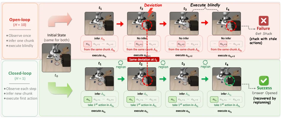
Figure 1 : Open-loop vs. Closed-loop execution. The top row ( H = 10 H=10 ) illustrates how blindly executing long action chunks leads to compounding errors, causing the robot to get stuck during a drawer-opening task. In contrast, the bottom row ( H = 1 H=1 ) demonstrates strict closed-loop execution, which maintains environmental reactivity and yields a smooth, successful manipulation.

Figure 1 presents the basic trade-off behind the paper. A longer action chunk reduces policy calls and improves efficiency, but keeps the robot open-loopThe controller commits to actions planned from the current observation and executes them without using later feedback to correct the remaining actions. for longer. In the top row, \(H=10\) means the robot blindly executes a longer chunk, so small errors compound and the drawer-opening task gets stuck. In the bottom row, \(H=1\) is close to strict closed-loopThe controller keeps observing during execution, compares what happened with what was expected, and updates future actions from that feedback. control: the robot observes and corrects at every step, preserving reactivity and completing the task. VLA-Corrector is designed to keep much of the long-chunk efficiency while recovering closed-loopThe controller keeps observing during execution, compares what happened with what was expected, and updates future actions from that feedback. correction when drift is detected.

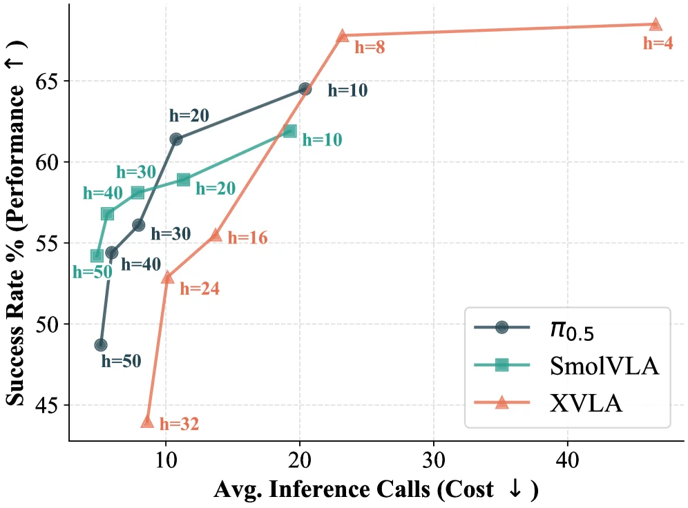
Figure 2 : Performance–efficiency trade-off across fixed action horizons. Smaller horizon achieves higher success rates, while larger horizon preserves the chunking efficiency.

This figure (Figure 2) illustrates the performance-efficiency tradeoff of three methods (π₀.₅, SmolVLA, XVLA) under different fixed action horizonThe number of consecutive future actions planned and executed from one policy call. A larger h executes a longer chunk with fewer model calls, but stays open-loop longer and can accumulate errors; a smaller h replans more often, improving reactivity at higher inference cost.s.

First, let’s examine the axes:
- The Y-axis represents "Success Rate %," where an upward arrow indicates improved performance—higher values mean more successful task execution.
- The X-axis represents "Avg. Inference Calls," where a downward arrow signifies reduced cost—lower values mean fewer calls to the policy model, resulting in higher efficiency.

Three curves appear in the graph, each representing a different method (distinguished by the legend):
1. π₀.₅ (dark blue dotted line with circles): Likely a baseline method or a specific configuration of a policy.
2. SmolVLA (teal line with squares): A method mentioned in the paper.
3. XVLA (orange line with triangles): An implementation or variant of VLA-Corrector, the main method proposed in the paper.

Each data point on the curves is labeled "h=some value," where "h" denotes the action horizonThe number of consecutive future actions planned and executed from one policy call. A larger h executes a longer chunk with fewer model calls, but stays open-loop longer and can accumulate errors; a smaller h replans more often, improving reactivity at higher inference cost.—the number of consecutive actions planned and executed in a single policy call. For example, "h=50" means one call executes 50 actions.

Analyzing Trends and Implications:

  • For all three methods, as the action horizonThe number of consecutive future actions planned and executed from one policy call. A larger h executes a longer chunk with fewer model calls, but stays open-loop longer and can accumulate errors; a smaller h replans more often, improving reactivity at higher inference cost. h increases (i.e., more actions are executed per call), the average number of inference calls decreases (moving left on the X-axis). This reflects improved chunking efficiency, as policy calls become less frequent.
  • However, as h increases, the success rate generally decreases (moving down on the Y-axis). This is because a larger action horizonThe number of consecutive future actions planned and executed from one policy call. A larger h executes a longer chunk with fewer model calls, but stays open-loop longer and can accumulate errors; a smaller h replans more often, improving reactivity at higher inference cost. means longer "open-loopThe controller commits to actions planned from the current observation and executes them without using later feedback to correct the remaining actions." execution, making the system less adaptable to environmental changes and more prone to accumulating errors, which increases the task failure rate. This is a limitation of the "predict-then-blindly-execute" paradigm.

Specific Method Behaviors:

  • XVLA (orange triangles): This curve is the highest and furthest to the right, indicating a strong balance between high success rates and low inference calls. For example, at h=8, it achieves a high success rate with relatively few calls. When h decreases to 4, the success rate drops slightly, but inference calls increase significantly.
  • SmolVLA (teal squares): Its performance lies between π₀.₅ and XVLA. Like XVLA, its success rate declines as h increases, but at the same h values, its success rate is typically lower than XVLA’s, while inference calls may be slightly higher or similar.
  • π₀.₅ (dark blue circles): At low h values (e.g., h=50), its success rate is low. However, as h increases (e.g., h=10, 20, 30), its success rate improves significantly, peaking at h=10. Beyond h=20, further increases in h yield diminishing or slightly decreasing returns in success rate.

Method Mechanics (From the Paper Abstract):

The proposed VLA-Corrector (XVLA in the figure) addresses the limitations of traditional fixed-action-horizon methods. It introduces a lightweight Latent Visual Monitor (LVM) to continuously compare predicted and actual visual feature evolution, detecting visual dynamics deviations online. When persistent deviations are detected, the system triggers a "truncation event," discards outdated actions, and performs corrective replanning via Online Gradient GuidanceOGG. During replanning, it turns the gap between expected and observed visual evolution into a corrective direction, nudging the generated action sequence back toward a recoverable trajectory without retraining the policy. (OGGOnline Gradient Guidance. A correction signal added during replanning: when execution has drifted, the model uses visual deviation to guide the next generated actions instead of blindly sampling a new chunk.).

Key Findings from the Figure:

  1. Fixed Action Horizon Tradeoff: All methods show that increasing h improves success rates (due to reduced inference calls and higher efficiency) but may decrease success rates (due to increased cumulative error risk with long horizons). This aligns with the "predict-then-blindly-execute" limitation noted in the abstract.
  2. VLA-Corrector Advantage: XVLA outperforms the others, especially at moderate to high h values. This demonstrates that VLA-Corrector’s event-triggered adaptive action horizonThe number of consecutive future actions planned and executed from one policy call. A larger h executes a longer chunk with fewer model calls, but stays open-loop longer and can accumulate errors; a smaller h replans more often, improving reactivity at higher inference cost. (maintaining long horizons when current actions are reliable, or triggering short-horizon corrections when execution drifts) effectively mitigates the tradeoff, achieving high success rates and chunking efficiency.
  3. Method Comparison: XVLA outperforms SmolVLA and π₀.₅ across most h values, particularly in balancing success rates and efficiency, validating VLA-Corrector’s effectiveness.

Conclusion:

The figure clearly illustrates the performance-efficiency tradeoff for three methods under varying fixed action horizonThe number of consecutive future actions planned and executed from one policy call. A larger h executes a longer chunk with fewer model calls, but stays open-loop longer and can accumulate errors; a smaller h replans more often, improving reactivity at higher inference cost.s. The key insight is that while larger h improves efficiency (fewer inference calls), it may sacrifice some success rate. However, VLA-Corrector (XVLA) optimizes this tradeoff through its adaptive horizon mechanism, achieving strong performance and efficiency. Data points (e.g., h=50, 40, 30, 20, 16, 10, 8, 4) highlight specific behaviors at different settings, aiding in understanding method suitability for various scenarios.

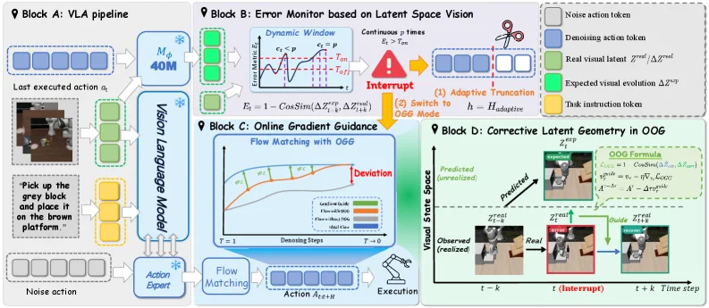
Figure 3 : Overview of VLA-Corrector. Starting from a standard chunked VLA pipeline ( A ), we add a Latent-space Vision Monitor (LVM) that detects persistent execution drift and triggers an interrupt event ( B ). The event truncates stale actions and switches the next replan from normal flow matching to OGG-guided flow matching ( C ). OGG uses the expected and observed latent evolution to guide the replan back toward a recoverable trajectory ( D ).

This diagram illustrates the overall architecture of the VLA-Corrector method, which we can understand through its workflow and methodological logic by dividing it into four main modules (Block A to Block D):

Block A: VLA Pipeline (Standard Chunked VLA Pipeline)

  • The "Last executed action \( a_t \)" (last action performed) and "Noise action" on the left serve as inputs to the "Vision Language Model." Additionally, a task instruction (e.g., "Pick up the grey block and place it on the brown platform") is also input into the vision language model.
  • The output of the vision language model is passed to the "Action Expert," which then generates a sequence of actions (the action sequence at the bottom of the diagram). The process here is the standard action chunking execution method: the model generates multiple future actions at once and executes them in an open-loopThe controller commits to actions planned from the current observation and executes them without using later feedback to correct the remaining actions. manner within a fixed action horizonThe number of consecutive future actions planned and executed from one policy call. A larger h executes a longer chunk with fewer model calls, but stays open-loop longer and can accumulate errors; a smaller h replans more often, improving reactivity at higher inference cost., meaning a "predict and blindly execute" mode.

Block B: Error Monitor Based on Latent Space Vision (Error Monitor Based on Latent Space Vision)

  • The role of this module is to detect execution drift. It receives information related to visual features from Block A (the green and blue blocks at the top of the diagram, possibly representing the evolution of real visual latent features \( z^v \) and predicted visual latent features \( \hat{z}^v \)).
  • First, there is a "Dynamic Window" where "\( E_t = 1 - \text{CosSim}(\Delta \hat{z}^v_t, \Delta z^v_t) \)" (the difference in cosine similarity, used to measure the difference between the predicted and actual visual feature evolution) is calculated. When this error \( E_t \) persistently exceeds a certain threshold (the red "Interrupt" trigger condition in the diagram, i.e., "persistent \( E_t > \tau_{\text{th}} \)"), an interrupt event is triggered.
  • The interrupt event triggers two operations: (1) "Adaptive Truncation," which discards the remaining "stale actions" (subsequent action sequences are cut off with scissors in the diagram); (2) "Switch to OGGOnline Gradient Guidance. A correction signal added during replanning: when execution has drifted, the model uses visual deviation to guide the next generated actions instead of blindly sampling a new chunk. Mode," which means switching from normal flow matchingA generative modeling method that learns a continuous path from noise or an intermediate state to the target sample. Here the target sample is a future robot action sequence; OGG adds a corrective guide to that generation path. to Online Gradient GuidanceOGG. During replanning, it turns the gap between expected and observed visual evolution into a corrective direction, nudging the generated action sequence back toward a recoverable trajectory without retraining the policy. (OGGOnline Gradient Guidance. A correction signal added during replanning: when execution has drifted, the model uses visual deviation to guide the next generated actions instead of blindly sampling a new chunk.) flow matchingA generative modeling method that learns a continuous path from noise or an intermediate state to the target sample. Here the target sample is a future robot action sequence; OGG adds a corrective guide to that generation path..

Block C: Online Gradient GuidanceOGG. During replanning, it turns the gap between expected and observed visual evolution into a corrective direction, nudging the generated action sequence back toward a recoverable trajectory without retraining the policy. (Online Gradient GuidanceOGG. During replanning, it turns the gap between expected and observed visual evolution into a corrective direction, nudging the generated action sequence back toward a recoverable trajectory without retraining the policy.)

  • This module starts working when Block B triggers an interrupt and switches to OGGOnline Gradient Guidance. A correction signal added during replanning: when execution has drifted, the model uses visual deviation to guide the next generated actions instead of blindly sampling a new chunk. mode. Its inputs include "Denoising steps" and "Flow Matching with OGGOnline Gradient Guidance. A correction signal added during replanning: when execution has drifted, the model uses visual deviation to guide the next generated actions instead of blindly sampling a new chunk.."
  • The curves in the diagram show the evolution of flow matchingA generative modeling method that learns a continuous path from noise or an intermediate state to the target sample. Here the target sample is a future robot action sequence; OGG adds a corrective guide to that generation path. under different situations (such as "OGGOnline Gradient Guidance. A correction signal added during replanning: when execution has drifted, the model uses visual deviation to guide the next generated actions instead of blindly sampling a new chunk.-guided," "Normal," etc.). When a deviation ("Deviation") is detected, OGGOnline Gradient Guidance. A correction signal added during replanning: when execution has drifted, the model uses visual deviation to guide the next generated actions instead of blindly sampling a new chunk. uses the expected and observed latent evolution to guide replanning, bringing the action sequence back to a recoverable trajectory. Here, "Action \( a_{t + \Delta t} \)" is the action corrected by OGGOnline Gradient Guidance. A correction signal added during replanning: when execution has drifted, the model uses visual deviation to guide the next generated actions instead of blindly sampling a new chunk. and then passed to the "Execution" module.

Block D: Corrective Latent Geometry in OGGOnline Gradient Guidance. A correction signal added during replanning: when execution has drifted, the model uses visual deviation to guide the next generated actions instead of blindly sampling a new chunk. (Corrective Latent Geometry in OGGOnline Gradient Guidance. A correction signal added during replanning: when execution has drifted, the model uses visual deviation to guide the next generated actions instead of blindly sampling a new chunk.)

  • This module shows the specific effect of the event-triggered adaptive action horizonThe number of consecutive future actions planned and executed from one policy call. A larger h executes a longer chunk with fewer model calls, but stays open-loop longer and can accumulate errors; a smaller h replans more often, improving reactivity at higher inference cost.. The timeline is divided into several stages: \( t - k \) (before the interrupt), \( t \) (at the time of the interrupt), and \( t + k \) (after the interrupt).
  • In the \( t - k \) stage, the system is in normal open-loopThe controller commits to actions planned from the current observation and executes them without using later feedback to correct the remaining actions. execution (the "OOO Formula" may represent the normal open-loopThe controller commits to actions planned from the current observation and executes them without using later feedback to correct the remaining actions. optimization formula), with predicted latent features \( z^v_{\text{pred}} \) and observed latent features \( z^v_{\text{obs}} \).
  • When a deviation is detected and an interrupt is triggered at time \( t \), the system enters the correction stage (the "OGGOnline Gradient Guidance. A correction signal added during replanning: when execution has drifted, the model uses visual deviation to guide the next generated actions instead of blindly sampling a new chunk. Formula" represents the optimization formula of Online Gradient GuidanceOGG. During replanning, it turns the gap between expected and observed visual evolution into a corrective direction, nudging the generated action sequence back toward a recoverable trajectory without retraining the policy.). By comparing the predicted and observed latent features, OGGOnline Gradient Guidance. A correction signal added during replanning: when execution has drifted, the model uses visual deviation to guide the next generated actions instead of blindly sampling a new chunk. guides replanning so that in the \( t + k \) stage, the actions can return to a path consistent with the real trajectory ("Real"), thus correcting the execution drift.

Overall Operating Logic of the Method

  1. Initial Execution: Start with the standard chunked VLA pipeline in Block A, where the model generates and executes a set of actions (open-loopThe controller commits to actions planned from the current observation and executes them without using later feedback to correct the remaining actions. execution).
  2. Error Detection: Block B continuously monitors the difference in evolution between predicted and actual visual features. When the error persistently exceeds the threshold, an interrupt is triggered.
  3. Interrupt Handling: After the interrupt is triggered, Block B discards the remaining stale actions and switches to OGGOnline Gradient Guidance. A correction signal added during replanning: when execution has drifted, the model uses visual deviation to guide the next generated actions instead of blindly sampling a new chunk. mode (Block C).
  4. Corrective Execution: Block C uses online gradient guidance to correct the action sequence, bringing the execution back to a recoverable trajectory (Block D shows the corrected latent geometry and trajectory, implementing an adaptive action horizonThe number of consecutive future actions planned and executed from one policy call. A larger h executes a longer chunk with fewer model calls, but stays open-loop longer and can accumulate errors; a smaller h replans more often, improving reactivity at higher inference cost.: when the current action chunk is reliable, maintain long-horizon execution; when execution starts to drift, trigger short-horizon corrective replanning).

In this way, the VLA-Corrector mitigates the lack of open-loopThe controller commits to actions planned from the current observation and executes them without using later feedback to correct the remaining actions. reactivity in the "predict and blindly execute" paradigm without modifying the weights of the backbone policy, solving the problem of task failure caused by the amplification of local disturbances in contact-rich physical interactions.

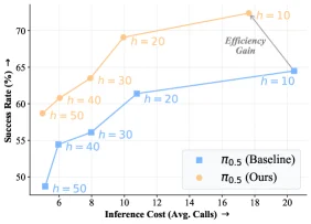
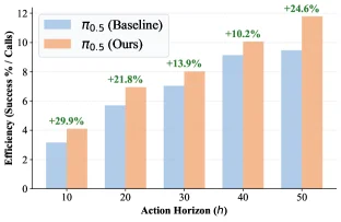
Figure 4 : Performance–efficiency analysis on π 0.5 \pi_{0.5} . Left : performance–efficiency trade-off across action horizons. Right : success-per-call efficiency. VLA-Corrector improves success rate across action horizons and yields consistent efficiency gains.

This figure (Figure 4) presents a performance - efficiency analysis of the VLA - Corrector method on the policy \(\boldsymbol{\pi_{0.5}}\). It focuses on comparing the "Our method (\(\pi_{0.5}\) (Ours), orange dot - line)" and "Baseline method (\(\pi_{0.5}\) (Baseline), blue dot - line)" in terms of success rate (vertical axis, %) and inference cost (horizontal axis, average number of calls) under different action horizonThe number of consecutive future actions planned and executed from one policy call. A larger h executes a longer chunk with fewer model calls, but stays open-loop longer and can accumulate errors; a smaller h replans more often, improving reactivity at higher inference cost.s (denoted by \(h\), e.g., \(h = 10, 20, 30, 40, 50\)), while also illustrating the efficiency gain.

Components of the Figure and Information Flow:

  • Horizontal Axis (Inference Cost): Represents the "average number of inference calls". A larger value means the strategy needs to call inference (or check/adjust after executing an action chunk) more frequently, but it may be more "efficient" (as it can correct errors in time); a smaller value means fewer calls, which is more "computation - saving" but may be more error - prone.
  • Vertical Axis (Success Rate): Represents the proportion of successful tasks (%). A higher value indicates that the strategy has a stronger ability to execute the task.
  • Two Curves:
  • Orange Curve (\(\pi_{0.5}\) (Ours)): Represents our VLA - Corrector method. As the action horizonThe number of consecutive future actions planned and executed from one policy call. A larger h executes a longer chunk with fewer model calls, but stays open-loop longer and can accumulate errors; a smaller h replans more often, improving reactivity at higher inference cost. \(h\) changes (from \(h = 50\) to \(h = 10\) or vice versa? Looking at the point labels: when \(h = 50\), the orange point is at the lower left (inference cost ≈ 6, success rate ≈ 58%); when \(h = 40\), (inference cost ≈ 8, success rate ≈ 61%); when \(h = 30\), (inference cost ≈ 10, success rate ≈ 64%); when \(h = 20\), (inference cost ≈ 12, success rate ≈ 69%); when \(h = 10\), (inference cost ≈ 18, success rate ≈ 72%). The overall trend is: **The smaller the action horizonThe number of consecutive future actions planned and executed from one policy call. A larger h executes a longer chunk with fewer model calls, but stays open-loop longer and can accumulate errors; a smaller h replans more often, improving reactivity at higher inference cost. \(h\) (i.e., the shorter the action chunk executed each time, or the more frequently the check/adjustment is performed), the higher the success rate tends to be? Wait, \(h = 10\) has a smaller \(h\) than \(h = 20\)? No, \(h\) is the action horizonThe number of consecutive future actions planned and executed from one policy call. A larger h executes a longer chunk with fewer model calls, but stays open-loop longer and can accumulate errors; a smaller h replans more often, improving reactivity at higher inference cost.. Maybe \(h = 10\) represents a "short action horizonThe number of consecutive future actions planned and executed from one policy call. A larger h executes a longer chunk with fewer model calls, but stays open-loop longer and can accumulate errors; a smaller h replans more often, improving reactivity at higher inference cost." (executing 10 steps or 10 actions at a time), and \(h = 50\) represents a "long action horizonThe number of consecutive future actions planned and executed from one policy call. A larger h executes a longer chunk with fewer model calls, but stays open-loop longer and can accumulate errors; a smaller h replans more often, improving reactivity at higher inference cost.". Looking at the curve, the orange curve (our method) has the highest success rate when \(h = 10\) (≈ 72%) and the lowest when \(h = 50\) (≈ 58%).
  • Blue Curve (\(\pi_{0.5}\) (Baseline)): Represents the baseline method. When \(h = 50\), (inference cost ≈ 6, success rate ≈ 48%); when \(h = 40\), (inference cost ≈ 8, success rate ≈ 54%); when \(h = 30\), (inference cost ≈ 10, success rate ≈ 56%); when \(h = 20\), (inference cost ≈ 12, success rate ≈ 61%); when \(h = 10\), (inference cost ≈ 20, success rate ≈ 64%). The trend is: The smaller the \(h\) (shorter action horizonThe number of consecutive future actions planned and executed from one policy call. A larger h executes a longer chunk with fewer model calls, but stays open-loop longer and can accumulate errors; a smaller h replans more often, improving reactivity at higher inference cost.), the higher the success rate as \(h\) decreases, but the overall success rate is lower than that of the orange curve (our method).

  • Arrow and "Efficiency Gain": The gray arrow in the figure points from the orange point of \(h = 10\) to the blue point of \(h = 10\), labeled "Efficiency Gain", which means that under the same action horizonThe number of consecutive future actions planned and executed from one policy call. A larger h executes a longer chunk with fewer model calls, but stays open-loop longer and can accumulate errors; a smaller h replans more often, improving reactivity at higher inference cost. \(h = 10\), our method (orange) has a higher success rate than the baseline (blue), and at the same time, the inference cost (horizontal axis) is lower? No, the inference cost of our method when \(h = 10\) is ≈ 18, and that of the baseline is ≈ 20. So our method, with a slightly lower inference cost (or similar), achieves a higher success rate, reflecting the "efficiency gain" — that is, our method optimizes the use of inference cost (or obtains a higher success with a lower cost) while maintaining or improving the success rate.

Operational Logic of the Method (Inferred from the Results):

The core of VLA - Corrector is the event - triggered adaptive action horizonThe number of consecutive future actions planned and executed from one policy call. A larger h executes a longer chunk with fewer model calls, but stays open-loop longer and can accumulate errors; a smaller h replans more often, improving reactivity at higher inference cost. of "detection - correction":
- When the execution of an action chunk (defined by the action horizonThe number of consecutive future actions planned and executed from one policy call. A larger h executes a longer chunk with fewer model calls, but stays open-loop longer and can accumulate errors; a smaller h replans more often, improving reactivity at higher inference cost. \(h\)) is "reliable" (i.e., the visual dynamic deviation is small), the method will retain the execution of the long action horizonThe number of consecutive future actions planned and executed from one policy call. A larger h executes a longer chunk with fewer model calls, but stays open-loop longer and can accumulate errors; a smaller h replans more often, improving reactivity at higher inference cost. (e.g., \(h = 20, 30\)) to reduce the number of inference calls (improve efficiency);
- When the execution starts to "drift" (the visual dynamic deviation persists), the method will trigger a truncation event: discard the remaining "stale" actions and perform corrective replanning through "Online Gradient GuidanceOGG. During replanning, it turns the gap between expected and observed visual evolution into a corrective direction, nudging the generated action sequence back toward a recoverable trajectory without retraining the policy. (OGGOnline Gradient Guidance. A correction signal added during replanning: when execution has drifted, the model uses visual deviation to guide the next generated actions instead of blindly sampling a new chunk.)". At this time, it will call the short action horizonThe number of consecutive future actions planned and executed from one policy call. A larger h executes a longer chunk with fewer model calls, but stays open-loop longer and can accumulate errors; a smaller h replans more often, improving reactivity at higher inference cost. (e.g., \(h = 10\)) for execution to improve the success rate.

From the results in the figure:
- Our method (orange) has a higher success rate than the baseline (blue) under all action horizonThe number of consecutive future actions planned and executed from one policy call. A larger h executes a longer chunk with fewer model calls, but stays open-loop longer and can accumulate errors; a smaller h replans more often, improving reactivity at higher inference cost.s \(h\), indicating that the "detection - correction" mechanism of VLA - Corrector effectively reduces the error accumulation in the "open - loop blind zone" and improves the task success rate.
- Under the same action horizonThe number of consecutive future actions planned and executed from one policy call. A larger h executes a longer chunk with fewer model calls, but stays open-loop longer and can accumulate errors; a smaller h replans more often, improving reactivity at higher inference cost. (e.g., \(h = 10\)), our method has a higher success rate and better efficiency (the "Efficiency Gain" labeled by the arrow), indicating that the method has achieved a better balance in the "success rate - efficiency" trade - off: it reduces computation by using a long horizon and corrects errors by using a short horizon, and ultimately improves the performance under various horizons, and has higher efficiency under a specific horizon (e.g., \(h = 10\)).

Conclusion (Drawn from the Figure):

Through the event - triggered adaptive action horizonThe number of consecutive future actions planned and executed from one policy call. A larger h executes a longer chunk with fewer model calls, but stays open-loop longer and can accumulate errors; a smaller h replans more often, improving reactivity at higher inference cost. (long horizon for efficiency, short horizon for error correction), VLA - Corrector achieves on the \(\pi_{0.5}\) policy:
1. Success Rate Improvement: The success rate is higher than that of the baseline method under all action horizonThe number of consecutive future actions planned and executed from one policy call. A larger h executes a longer chunk with fewer model calls, but stays open-loop longer and can accumulate errors; a smaller h replans more often, improving reactivity at higher inference cost.s (\(h = 10, 20, 30, 40, 50\));
2. Efficiency Gain: Under the same action horizonThe number of consecutive future actions planned and executed from one policy call. A larger h executes a longer chunk with fewer model calls, but stays open-loop longer and can accumulate errors; a smaller h replans more often, improving reactivity at higher inference cost. (e.g., \(h = 10\)), the improvement of the success rate is accompanied by the optimization of the inference cost (or a higher success is obtained with a lower cost), alleviating the "success rate - efficiency" trade - off of the "prediction - blind execution" paradigm.

In short, the figure clearly shows that VLA - Corrector can improve the success rate of the strategy under different action horizonThe number of consecutive future actions planned and executed from one policy call. A larger h executes a longer chunk with fewer model calls, but stays open-loop longer and can accumulate errors; a smaller h replans more often, improving reactivity at higher inference cost.s and has a higher efficiency (the balance between success rate and inference cost) than the baseline method.

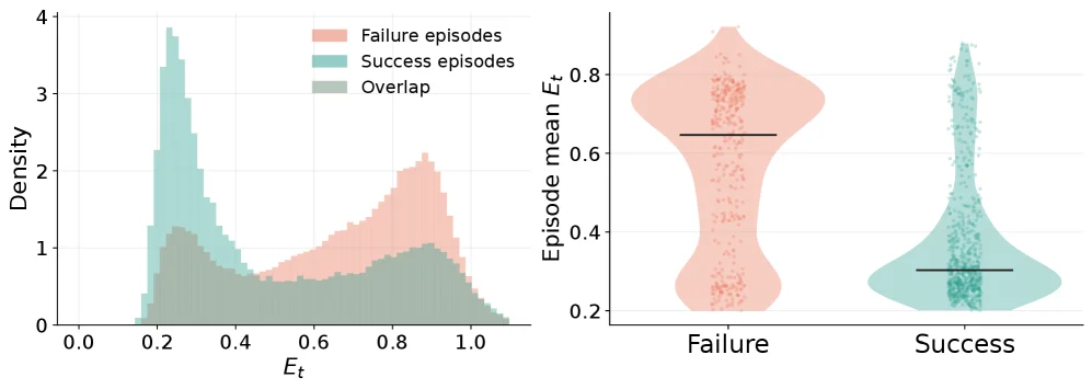
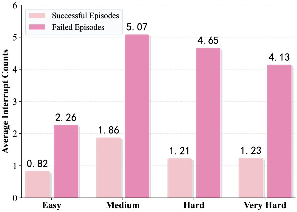
Figure 5 : LVM detection analysis. Left : distribution of the inconsistency score E t E_{t} , where successful episodes concentrate at low values and failed episodes show a heavier high-score tail. Right : interrupt frequency, where failed episodes trigger more interrupt events than successful ones.

Figure 5 checks whether the Latent-space Vision Monitor (LVM) actually detects meaningful execution errors. The left plot shows the inconsistency score \(E_t\): successful episodes concentrate at low scores, while failed episodes have a heavier high-score tail. The right plot shows interrupt frequency: failed episodes trigger more interrupts than successful ones. Together, these results indicate that LVM interrupts are correlated with real execution drift rather than random noise.

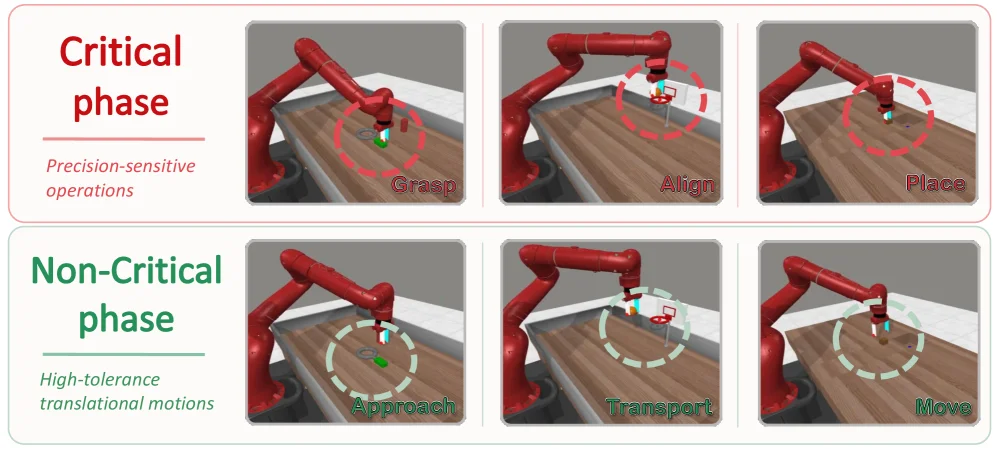
Figure 6 : Task-phase analysis of LVM-triggered truncation. We manually divide MetaWorld trajectories into critical and non-critical phases. Left : representative trajectories show that truncation is triggered much more frequently during critical phases. Right : 83.7% of truncations occur in critical phases, while only 16.3% occur in non-critical phases.

Figure 6 analyzes when LVM-triggered truncation happens. The authors manually divide MetaWorld trajectories into critical and non-critical phases. Critical phases are moments such as contact, grasping, insertion, or placement, where a small deviation can cause failure. The examples and statistics show that 83.7% of truncations occur in critical phases and only 16.3% in non-critical phases, suggesting that the monitor tends to interrupt when correction is actually needed.

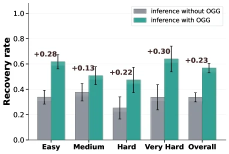
Figure 7 : Post-interrupt recovery. OGG-guided inference consistently outperforms standard inference.

Figure 7 compares recovery after an interrupt. Standard inference replans from the current state but does not explicitly use the detected visual deviation as a correction direction. OGGOnline Gradient Guidance. A correction signal added during replanning: when execution has drifted, the model uses visual deviation to guide the next generated actions instead of blindly sampling a new chunk.-guided inference turns the gap between expected and observed visual evolution into guidance for the new action sequence. The result shows that OGGOnline Gradient Guidance. A correction signal added during replanning: when execution has drifted, the model uses visual deviation to guide the next generated actions instead of blindly sampling a new chunk.-guided inference consistently recovers better than standard inference in the post-interrupt setting.

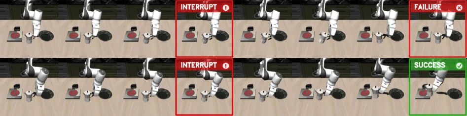
Figure 8 : Controlled recovery case. Given the same initial state and detected grasping error, the monitored baseline continues the original chunk and fails ( top ), while VLA-Corrector truncates stale actions, replans with OGG, and completes the task ( bottom ).

This figure (Figure 8) is a visual comparison of a "controlled recovery case," designed to clearly demonstrate the different behaviors of the proposed VLA-Corrector method and a traditional baseline method when handling errors that occur during execution.

First, let's analyze the structure of the image. The entire image is divided into two rows, each representing a different execution scenario or method. Each row consists of multiple consecutive scene snapshots, which are arranged in chronological order from left to right, illustrating the task execution process.

The top row (labeled with red boxes) represents the "monitored baseline" method: 1. Initial Phase (the leftmost few snapshots): This part shows the initial state of the task, where the robot arm and target objects (such as a red disk and a gray cylinder) are in their starting positions. These snapshots appear identical to those in the corresponding positions of the bottom row, indicating that both methods share the same initial conditions and the first few steps of execution are consistent. 2. Error Detection and Failure (middle red box labeled "INTERRUPT" and the rightmost red box labeled "FAILURE"): * At a certain point (marked by the red box labeled "INTERRUPT"), the system detects an error. Visually, this might indicate that the robot failed to grasp the object correctly, or the object's position deviates from what was expected. * Despite detecting the error, the "monitored baseline" method continues to execute the pre-planned sequence of actions (i.e., the remaining actions in the "chunk"). We can see that the robot arm's movements do not correct the error but continue according to the original plan. * Ultimately, in the rightmost snapshot (labeled "FAILURE"), the task ends in failure. Visually, this might mean the object was not placed correctly at the target location, or the robot arm is in an invalid state.

The bottom row (labeled with a green box) represents the "VLA-Corrector" method: 1. Initial Phase (the leftmost few snapshots): Similar to the top row, this part shows the initial state of the task and the first few steps of execution, which are consistent between the two methods. 2. Error Detection and Recovery (middle red box labeled "INTERRUPT" and the rightmost green box labeled "SUCCESS"): * At a similar point (marked by the red box labeled "INTERRUPT"), the system also detects an error, which appears similar to the one detected by the baseline method (e.g., a grasping error). * However, the VLA-Corrector method takes a different approach. Instead of continuing to execute the remaining, potentially unreliable, actions in the sequence, it "truncates" the current sequence of actions (i.e., discards the stale actions remaining in the "chunk"). * Subsequently, VLA-Corrector performs replanning through "Online Gradient GuidanceOGG. During replanning, it turns the gap between expected and observed visual evolution into a corrective direction, nudging the generated action sequence back toward a recoverable trajectory without retraining the policy." (OGGOnline Gradient Guidance. A correction signal added during replanning: when execution has drifted, the model uses visual deviation to guide the next generated actions instead of blindly sampling a new chunk.). Visually, the robot arm's actions change; it begins to execute a new, corrected sequence of actions. * Finally, in the rightmost snapshot (labeled "SUCCESS"), the task is successfully completed. Visually, this means the object has been correctly placed at the target location, or the robot arm has reached the desired successful state.

Mechanism of the method revealed by the image: This image intuitively illustrates the core idea of VLA-Corrector: * Detect: The system can monitor visual dynamic deviations online (as indicated by the "INTERRUPT" marker) to identify errors or drifts during execution. * Truncate: Once a persistent deviation is detected, the system truncates the currently executing, potentially obsolete, sequence of actions (i.e., discards the remaining actions in the "chunk"). * Correct: The system invokes "Online Gradient GuidanceOGG. During replanning, it turns the gap between expected and observed visual evolution into a corrective direction, nudging the generated action sequence back toward a recoverable trajectory without retraining the policy." (OGGOnline Gradient Guidance. A correction signal added during replanning: when execution has drifted, the model uses visual deviation to guide the next generated actions instead of blindly sampling a new chunk.) for replanning, generating a new, more appropriate sequence of actions. * Adaptive Action Horizon: VLA-Corrector dynamically adjusts the execution horizon based on the execution status. It maintains a longer execution horizon when the current action sequence is reliable, and invokes a shorter-horizon corrective replanning when execution starts to deviate from expectations.

Comparison Objects and Conclusion: * Comparison Objects: The image directly compares two methods: the "monitored baseline" method (top row) and the "VLA-Corrector" method (bottom row). * Coordinates/Order: Time flows from left to right, with each snapshot representing a time step. * Conclusion: The figure clearly shows that, given the same initial state and a detected grasping error, the "monitored baseline" method leads to task failure because it continues to execute the erroneous action sequence. In contrast, the VLA-Corrector method successfully recovers from the error by truncating stale actions and performing replanning, thus completing the task. This demonstrates the effectiveness of the VLA-Corrector method in improving the robustness and adaptability of embodied agents in contact-rich physical interaction tasks.

In summary, this figure, through a specific case, vividly demonstrates how the VLA-Corrector method achieves task recovery when encountering execution errors through its "detect-truncate-correct" mechanism, thereby overcoming the limitations of traditional baseline methods.

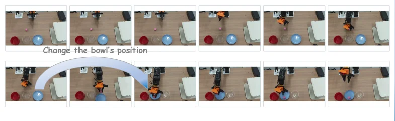
Figure 9 : Real-world disturbance recovery demo. A human shifts the blue bowl during execution, requiring the robot to recover from an outdated action chunk.

This figure demonstrates a real-world disturbance recovery scenario, where a robot (the orange manipulator arm) needs to recover from an outdated action chunk when an unexpected environmental change occurs (a human shifts the blue bowl) during task execution.

We can understand the image by dividing it into two main rows:

Upper Row of Images (left to right): * This part shows the initial planning and execution phase of the task. * Initially, the robot executes a sequence of actions based on its plan (possibly a pre-defined action chunk), interacting with objects on the table (a red bowl, a blue bowl, a transparent small bowl, and a pink ball). * The images show the robot sequentially performing actions, such as moving above the blue bowl, seemingly intending to manipulate it (e.g., grasp or move it). * The key point is that these actions are executed based on an "outdated action chunk," meaning the environment was in a certain state when the robot started executing this sequence, but the environment changes during execution.

Key Disturbance (text and arrow): * Below the upper row of images, there is text that reads "Change the bowl's position," accompanied by a large blue arrow pointing from left to right. * This arrow and text clearly indicate that during the robot's execution of the aforementioned action sequence (approximately in the middle to later part of the upper row), an external disturbance occurs: a human moves the blue bowl. * This disturbance renders the robot's originally planned actions obsolete because they were based on an old environmental state.

Lower Row of Images (left to right): * This part shows how the VLA-Corrector method detects the disturbance and performs recovery. * After the robot completes the action chunk from the upper sequence (or during its execution), the "Latent-space Vision Monitor (LVM)" of VLA-Corrector continuously compares the predicted visual feature evolution with the actual visual feature evolution. * Once a persistent deviation is detected (i.e., the actual environment no longer matches the predicted environment, such as the blue bowl's position having changed), the system triggers a "truncation event." * The truncation event discards the remaining, potentially obsolete actions and invokes corrective replanning via "Online Gradient GuidanceOGG. During replanning, it turns the gap between expected and observed visual evolution into a corrective direction, nudging the generated action sequence back toward a recoverable trajectory without retraining the policy. (OGGOnline Gradient Guidance. A correction signal added during replanning: when execution has drifted, the model uses visual deviation to guide the next generated actions instead of blindly sampling a new chunk.)." * The lower row of images shows the robot readjusting its actions based on the new environmental state (the blue bowl has been moved) and continuing to complete the task (e.g., it might still be manipulating the pink ball, but now needs to account for the blue bowl's new position).

How the Method Works: 1. Initial Planning and Execution: The robot executes a sequence of actions based on a pre-defined action chunk (as shown in the upper row). 2. Environmental Disturbance: During execution, the environment changes (e.g., a human moves the blue bowl). 3. Deviation Detection: VLA-Corrector's LVM detects a persistent deviation between the predicted visual state and the actual visual state. 4. Truncation and Replanning: Upon detecting the deviation, the system triggers a truncation event, discards the remaining old actions, and performs corrective replanning using OGGOnline Gradient Guidance. A correction signal added during replanning: when execution has drifted, the model uses visual deviation to guide the next generated actions instead of blindly sampling a new chunk.. 5. Adapting to the New Environment: The robot executes actions based on the new plan (as shown in the lower row) to adapt to the changed environment and successfully complete the task.

Conclusion: This figure clearly illustrates the core idea of the VLA-Corrector method: when an environmental disturbance renders an existing action chunk obsolete, the method can detect this deviation online and perform corrective replanning in a timely manner, allowing the robot to recover from the disturbance and continue executing the task successfully. It reveals how VLA-Corrector addresses the lack of closed-loopThe controller keeps observing during execution, compares what happened with what was expected, and updates future actions from that feedback. reactivity in traditional action-chunk mechanisms during open-loopThe controller commits to actions planned from the current observation and executes them without using later feedback to correct the remaining actions. execution through an event-triggered adaptive action horizonThe number of consecutive future actions planned and executed from one policy call. A larger h executes a longer chunk with fewer model calls, but stays open-loop longer and can accumulate errors; a smaller h replans more often, improving reactivity at higher inference cost..

This figure is not a traditional coordinate plot or comparison chart but a process demonstration diagram, showing the application process and effect of the method in a real-world scenario.

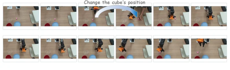
Figure 10 : Demo: Moving-object grasp. The robot picks up the cube and places it into the white bowl, while a human manually changes the cube’s position during the process.

Figure 10 is a real-world moving-object grasp demo. The robot must pick up a cube and place it into the white bowl, while a human changes the cube position during execution. That change makes the remaining actions in the old chunk stale. VLA-Corrector should detect the visual mismatch, truncate the stale chunk, and replan from the cube's new position so the task can continue.

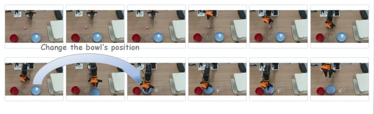
Figure 11 : Demo: Moving-placement target. The robot picks up the cube and places it into the blue bowl, while a human manually changes the bowl’s position during the process.

Figure 11 shows a moving placement target. The robot is asked to place the cube into the blue bowl, but a human moves the blue bowl during execution. A fixed action-chunk policy may keep moving toward the old target location. VLA-Corrector instead detects the target displacement, discards outdated actions, and replans actions that place the cube into the bowl at its new position.

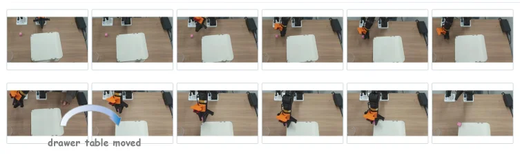
Figure 12 : Demo: Moving-insertion target. The robot picks up the cube and places it at the upper-left corner of the drawer top, while a human manually changes the drawer’s position during the process.

Figure 12 shows a moving insertion target. The robot must place the cube at the upper-left corner of the drawer top, while a human changes the drawer position. This kind of contact-rich placement is sensitive to the target pose, so stale actions can easily fail. The demo illustrates the detect-truncate-correct loop under a real disturbance: detect the mismatch, interrupt the obsolete chunk, and use OGGOnline Gradient Guidance. A correction signal added during replanning: when execution has drifted, the model uses visual deviation to guide the next generated actions instead of blindly sampling a new chunk.-guided replanning for the new drawer position.

← → flip · ↑ ↓ scroll notes · Esc exit