🌊 Tide

Information moves like the tide. We pick the waves worth studying.

中文

← Today's tide

Published 2026-06-30 · OMRON SINIC X Corp. · Bao Long Nguyen Huu, Atsushi Hashimoto

AGE: Adaptive-masking for Graph Embedding in Graph Retrieval-Augmented Generation

arXiv · HuggingFace · ▲2

Abstract (verbatim)

GraphRAG is an extension of retrieval-augmented generation (RAG) that supports large language models (LLMs) by referring to graph-structured data as external knowledge. While this technique ideally captures intricate relationships, it often struggles with graph representations for LLMs, particularly for frozen LLMs, due to the misalignment between graph-based and text-based latent features. We tackle this issue by introducing the {\it Adaptive-masking for Graph Embedding (AGE)}. AGE employs a Transformer in a mask-based self-supervised learning (SSL) approach. We designed the architecture similar to text embedding encoders, addressing the latent feature misalignment. In contrast to natural language texts, graphs are concise representations, and there exist {\it key nodes} that hold dominant contextual information, which are challenging to predict from their surroundings. Masking such key nodes leads to inefficiency in the SSL process. Therefore, AGE focuses on predicting nodes apart from key nodes, utilizing a learnable node sampler. Our experimental results indicate that AGE significantly improves approaches using non-parametric search component in GraphQA tasks, achieving superior accuracy across four benchmark datasets with distinct characteristics.

Background

Background Analysis

1. Technical Context
Large Language Models (LLMs) like GPT and Claude have advanced natural language understanding, but they struggle to access domain-specific structured knowledge (e.g., entity relationships in graphs) without retraining. Retrieval-Augmented Generation (RAG) addresses this by supplementing LLMs with external data, but traditional RAG fails to capture complex relationships effectively. Graph-Retrieval Augmented Generation (GraphRAG) improves this by using graph-structured data (nodes and edges) to represent relationships intuitively, which is useful in fields like healthcare or law (e.g., linking diseases to symptoms or regulations to cases). However, aligning graph structures with LLMs’ text-based representations remains challenging.

2. Previous Limitations
Existing approaches face two main issues:
- High Cost vs. Efficiency Tradeoff: Fine-tuning LLMs improves performance but is resource-intensive, while non-parametric retrievers (e.g., graph-based neural retrievers) are efficient but may miss critical nodes or include redundant information.
- Feature Misalignment: Graph embeddings often fail to match LLMs’ text-based feature spaces, leading to poor performance. For example, randomly masking nodes during self-supervised learning (SSL) disrupts key entities, degrading representation quality.

3. Proposed Solution
This paper introduces Adaptive-masking for Graph Embedding (AGE) to address these issues:
- Text-like Embedding Mechanism: AGE mimics LLMs’ mask-based SSL (e.g., RoBERTa) to align graph and text feature spaces, ensuring graph embeddings are interpretable by LLMs.
- Selective Node Masking: A reinforcement learning (RL)-trained sampler identifies "key nodes" (core entities) and masks only "auxiliary nodes" (secondary relationships), preserving graph integrity.
- JEPA Integration: The Joint-Embedding Predictive Architecture (JEPA) optimizes representations by eliminating redundant details, improving retrieval efficiency.

4. Key Differences
Unlike prior work, AGE:
- Optimizes Frozen LLMs: It enhances graph embeddings without fine-tuning LLMs, reducing computational costs.
- Adaptive Masking Strategy: RL-guided masking outperforms random masking by preserving critical nodes.
- Efficient Non-Parametric Retrieval: It achieves state-of-the-art (SOTA) results on benchmarks while maintaining low resource usage.

This approach provides a more accurate and efficient solution for GraphRAG in complex tasks like graph-based question answering.
Method, Figure by Figure

M E T H O D1 / 5

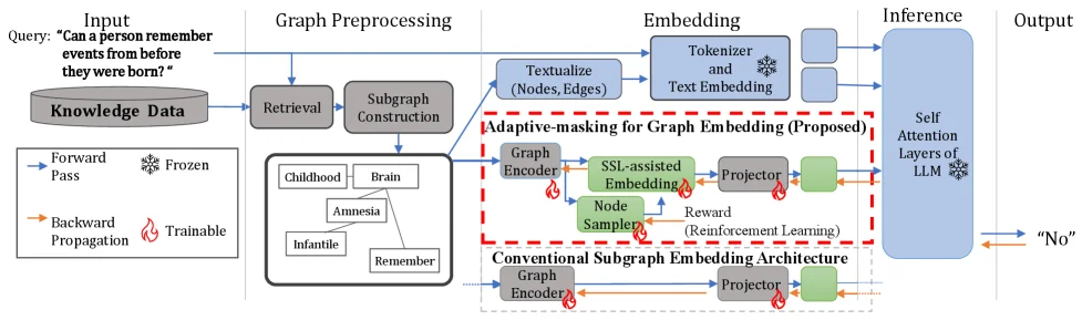
Figure 1 : Overview of GraphRAG with the proposed Adaptive-masking for Graph Embedding (AGE) embedding. 1) Retrieval: Find graph elements relevant to the query using a non-parametric process. 2) Subgraph Construction: Extend retrieved graph elements with their adjacencies [ G-Retriever ] . 3) Embedding: Use tokenizer and text embedder for textualized graph and query. Apply AGE for structured relationships of the graph. 4) Inference: Input embeddings into LLM to generate an answer.

This figure illustrates the overall workflow of the GraphRAG framework proposed in the paper "AGE: Adaptive-masking for Graph Embedding in Graph Retrieval-Augmented Generation," with a particular focus on its core innovation, Adaptive-masking for Graph Embedding (AGE).

Starting from the left side of the image, the input is a "Query," for example, the one shown: "Can a person remember events from before they were born?" This query is directed towards a "Knowledge Data" database. The data flow begins with the "Retrieval" module, which uses a non-parametric process to find graph elements relevant to the query. This corresponds to the first step in the caption: retrieving relevant graph elements.

Next is the "Subgraph Construction" module. Its function is to expand the retrieved graph elements by including their adjacencies, forming a more complete subgraph, as indicated by "G-Retriever" in the caption (step 2). The figure represents this subgraph with a diagram containing nodes like "Childhood," "Brain," "Amnesia," "Infantile," and "Remember."

The data then flows into the "Embedding" stage. This stage has two main paths: 1. Text Path: The subgraph and query first go through a "Textualize (Nodes, Edges)" process, converting the graph structure into text format. Then, this text is passed through a "Tokenizer and Text Embedding" module, which converts it into vector representations. This part of the processing is similar to traditional RAG methods. 2. Graph Structure Path (Core Innovation: AGE): This is the path highlighted by the red dashed box labeled "Adaptive-masking for Graph Embedding (Proposed)." This path aims to address the misalignment between graph-structured and text-based latent features, especially for frozen Language Models (LLMs). * First, the subgraph enters the "Graph Encoder." * Then, it utilizes a "Learnable Node Sampler" to select nodes for processing. According to the paper, AGE focuses on predicting non-key nodes because key nodes hold dominant contextual information and are challenging to predict from their surroundings. Directly masking key nodes would lead to inefficiency in the SSL process. * Next, an "SSL-assisted Embedding" module is used. This SSL (Self-Supervised Learning) approach is designed to be similar to text embedding encoders, addressing the misalignment issue. * The embedding result is then passed through a "Projector" to match the input requirements of subsequent modules. * The figure also shows a feedback loop labeled "Reward (Reinforcement Learning)," suggesting that reinforcement learning might be involved in optimizing the node sampling or embedding strategy.

Below the "Embedding" stage, there is a comparative section labeled "Conventional Subgraph Embedding Architecture." It also includes a "Graph Encoder" and a "Projector" but lacks the innovative components of AGE (like the learnable node sampler and SSL-assisted embedding), highlighting the improvements introduced by AGE.

Finally, all processed embeddings (from both the text path and the AGE graph path) are fed into the "Inference" stage, specifically the "Self Attention Layers of LLM." The LLM in this context has "Frozen" parameters, meaning its weights are not updated during inference. The LLM combines this embedded information to generate the final "Output," which in the example is "No."

Arrows in the diagram indicate the direction of data or information flow. A legend explains the different types of arrows: blue arrows represent "Forward Pass," orange arrows represent "Backward Propagation," the snowflake icon indicates "Frozen" (parameters not updated), and the flame icon indicates "Trainable" (parameters will be updated).

In summary, this figure clearly demonstrates how the GraphRAG framework processes a query by retrieving relevant graph data, constructing a subgraph, and then processing this graph data through both a traditional text embedding path and an innovative Adaptive-masking for Graph Embedding (AGE) path. The embeddings from these paths are then combined and fed into a frozen LLM for inference to generate an answer. The core of AGE lies in using SSL and a learnable node sampler to better align the latent features of graphs and text, thereby improving the performance of frozen LLMs in graph-based knowledge-augmented tasks.

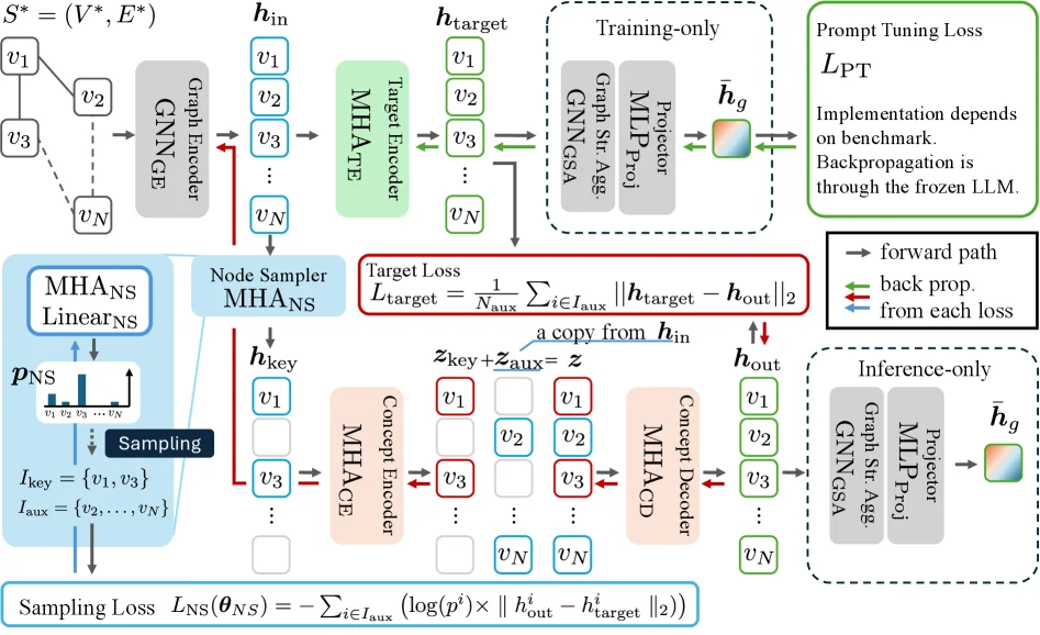
Figure 2 : Architecture for Adaptive-masking for Graph Embedding: During training, 𝒉 target {\bm{h}}_{\text{target}} is connected to the downstream for the target encoder training, while 𝒉 out {\bm{h}}_{\text{out}} is used during inference. The node sampler explores the optimal distribution for mask-based SSL for graphs. The loss functions train distinct sets of modules without overlap.

This diagram illustrates the architecture of the "Adaptive-masking for Graph Embedding (AGE)" method proposed in the paper "AGE: Adaptive-masking for Graph Embedding in Graph Retrieval-Augmented Generation." The method aims to address the mismatch between graph representations and the latent features of language models (especially frozen language models) in Graph Retrieval-Augmented Generation (GraphRAG).

Data Flow and Component Analysis:

  1. Input and Initial Encoding (Top Left):

    • The graph structure S* = (V*, E*) is input, where V* is the set of nodes (e.g., v1, v2, ..., vN) and E* is the set of edges.
    • This graph data is first passed through a Graph Encoder (GNNE) (Graph Neural Network Encoder), generating initial node representations h_in. h_in is a sequence of vectors, each corresponding to the representation of a node (v1 to vN).
  2. Target Encoder and Training Path (Upper Middle):

    • A part (or all, depending on the masking strategy) of h_in is fed into the Target Encoder (MHATE) (Target Encoder, where MHATE might stand for Multi-Head Attention Target Encoder). After processing by this encoder, h_target, the target node representations, is obtained.
    • During the training phase, h_target flows into a "Training-only" module, which includes GNN Str Agg (Graph Neural Network Structure Aggregation), MLP Proj (Multi-Layer Perceptron Projection), and Projector. The final output is ĝ. This ĝ is used to calculate the Prompt Tuning Loss (L_PT). The implementation of this loss depends on benchmarks, and backpropagation is performed through a frozen LLM.
  3. Node Sampler (Middle Left):

    • The Node Sampler (MHA_NS, Linear_NS) is one of the core components of AGE. It generates a sampling distribution p_NS based on h_in.
    • The sampling process determines two sets of nodes: I_key (the key node set, e.g., I_key = {v1, v3} in the figure) and I_aux (the auxiliary node set, e.g., I_aux = {v2, ..., vN} in the figure). Key nodes are considered to contain dominant contextual information and are difficult to predict from their surroundings, while auxiliary nodes are used for prediction.
  4. Masked Self-Supervised Learning (Middle):

    • Based on the sampled I_aux, the node representations in h_in corresponding to I_aux (e.g., h_in for v2, ..., vN in the figure) are fed into the Concept Encoder (MHACE) (Concept Encoder). Meanwhile, the node representations in h_in corresponding to I_key (h_in for v1, v3) are taken as z_key.
    • The Concept Decoder (MHACD) receives the output from MHACE (forming z by combining z_key and z_aux) and the representations of the I_key nodes in h_in (as conditions or references), and attempts to reconstruct h_out, the predicted representations of the auxiliary nodes.
    • Target Loss (L_target): Calculates the difference between h_target (from the target encoder) and h_out (from the concept decoder). This loss is used to train the target encoder and modules related to the concept encoder/decoder.
    • Sampling Loss (L_NS(θ_NS)): This loss is related to the node sampler. It optimizes the sampler's parameters θ_NS based on the sampling probability p_NS and the difference between h_out and h_target to find the optimal masking strategy.
  5. Inference Path (Bottom Right):

    • During the inference phase, h_out (from the concept decoder) is used instead of h_target. h_out also flows into the same downstream components in the "Training-only" module (GNN Str Agg, MLP Proj, Projector), and the final output ĝ is used for downstream tasks (such as graph retrieval or question answering).

Method Operation Mechanism:

  • Core Idea: AGE trains graph embeddings using a masked self-supervised learning method to address the mismatch between graph representations and the latent features of LLMs. Instead of randomly masking nodes, it focuses on predicting non-key nodes (auxiliary nodes) because key nodes are information-rich and difficult to predict.
  • Node Sampling: The node sampler learns a distribution to determine which nodes are key (should not be masked or used for prediction) and which are auxiliary (used for masked prediction). This is optimized through the sampling loss.
  • Dual Encoder Structure: The target encoder processes the original graph information to generate the target representation h_target, while the concept encoder and decoder process the masked auxiliary node information and attempt to reconstruct h_out.
  • Loss Functions: The target loss ensures that h_out is as close as possible to h_target, thus learning effective graph representations. The sampling loss optimizes the node sampling strategy to improve the efficiency of the SSL process.
  • Downstream Applications: The trained graph representations (h_out or ĝ obtained through the Projector) can be input as external knowledge into an LLM for graph retrieval augmentation generation tasks.

Summary: This diagram details the architecture of the AGE method, including the entire process from graph input to the generation of the final representation. It emphasizes the core idea of solving the mismatch between graph representations and LLMs through adaptive node sampling and masked self-supervised learning. By separating key nodes from auxiliary nodes and focusing on predicting the latter, AGE aims to learn more effective graph embeddings to improve the performance of GraphRAG in various tasks.

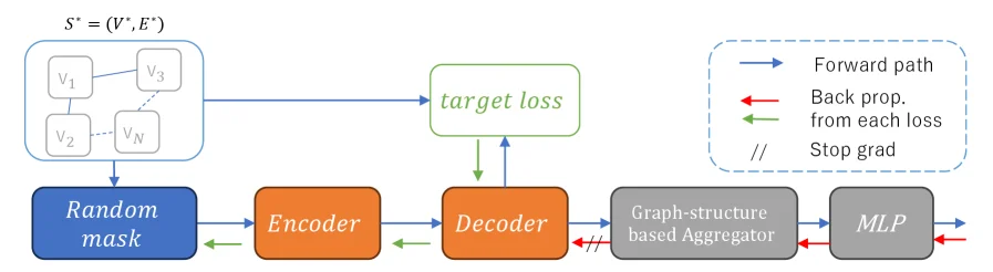
Figure H.7 : Adaptive-masking for Graph Embedding in Generation Architecture: The node embedding module is trained on both prompt tuning loss and target loss.

This diagram illustrates the "Adaptive-masking for Graph Embedding in Generation Architecture" proposed in the paper AGE: Adaptive-masking for Graph Embedding in Graph Retrieval-Augmented Generation. The core of this architecture is a node embedding module trained through prompt tuning loss and target loss.

Let’s break down each component and its data flow in the diagram:

1. Input Graph Structure (S* = (V, E))

The top-left of the diagram shows a graph structure S, where V represents the set of nodes (e.g., v₁, v₂, v₃, ..., vₙ) and E* represents the set of edges. This is the input data—the structured knowledge (graph) to be processed.

2. Random Mask

The input graph first passes through a "Random Mask" module. This module selects a subset of nodes to mask based on a learned strategy (a "learnable node sampler" in the paper). Unlike random masking all nodes, AGE focuses on masking "non-critical nodes"—since critical nodes’ information is hard to predict from their context, masking them directly would reduce self-supervised learning efficiency. Thus, this module identifies target nodes for prediction.

3. Encoder

The masked graph (or node features) is fed into the Encoder, which functions like a text embedding encoder: it converts graph nodes into low-dimensional vector representations (embeddings). This step is critical for the model to learn node features.

4. Decoder

The node embeddings from the encoder are passed to the Decoder, which predicts the masked nodes’ features/labels using context from unmasked nodes and the masked nodes’ surroundings. This is a classic self-supervised learning task.

5. Target Loss

The decoder’s predictions are compared to the true node information (or targets) to compute the Target Loss. This loss measures prediction accuracy and guides learning. Arrows show the loss backpropagates to update the decoder and encoder.

6. Graph-Structure Based Aggregator

After the decoder, the Graph-Structure Based Aggregator fuses the decoded node embeddings with the original graph’s structural information (e.g., adjacency). This step leverages graph structure to enhance node representations.

7. MLP (Multi-Layer Perceptron)

The aggregator’s output is fed into an MLP, which applies nonlinear transformations to the aggregated features—often for generating final outputs or supporting prompt tuning.

8. Prompt Tuning Loss

While not explicitly labeled, the MLP’s output (or an intermediate result) computes the Prompt Tuning Loss. This loss aligns embeddings with downstream tasks (e.g., graph retrieval-augmented generation).

9. Data Flow & Gradient Flow

  • Forward Path (Blue Arrows): Data flows from Input GraphRandom MaskEncoderDecoderGraph-Structure AggregatorMLP (model processes input to generate output).
  • Backpropagation (Red Arrows): Gradients flow backward from Target Loss to the decoder/encoder, and (implicitly) from Prompt Tuning Loss to the MLP/aggregator (to update parameters).
  • From Each Loss (Green Arrows): Shows how Target Loss backpropagates to the encoder.
  • Stop Grad (//): Indicates gradient flow stops at the decoder→aggregator connection. This isolates training objectives or prevents interference between components.

How AGE Works (Summary)

  1. A graph structure is input.
  2. A learnable strategy (Random Mask) selects "non-critical" nodes to mask.
  3. The partially masked graph is encoded into node embeddings.
  4. The decoder reconstructs masked nodes; errors (via Target Loss) update the encoder/decoder.
  5. Decoded embeddings are fused with graph structure (via the aggregator) and passed to an MLP.
  6. The MLP’s output computes Prompt Tuning Loss, optimizing embeddings for downstream tasks.

This self-supervised process trains the node embedding module by minimizing both Target Loss and Prompt Tuning Loss, improving alignment between graph and text features while efficiently learning from non-critical nodes.

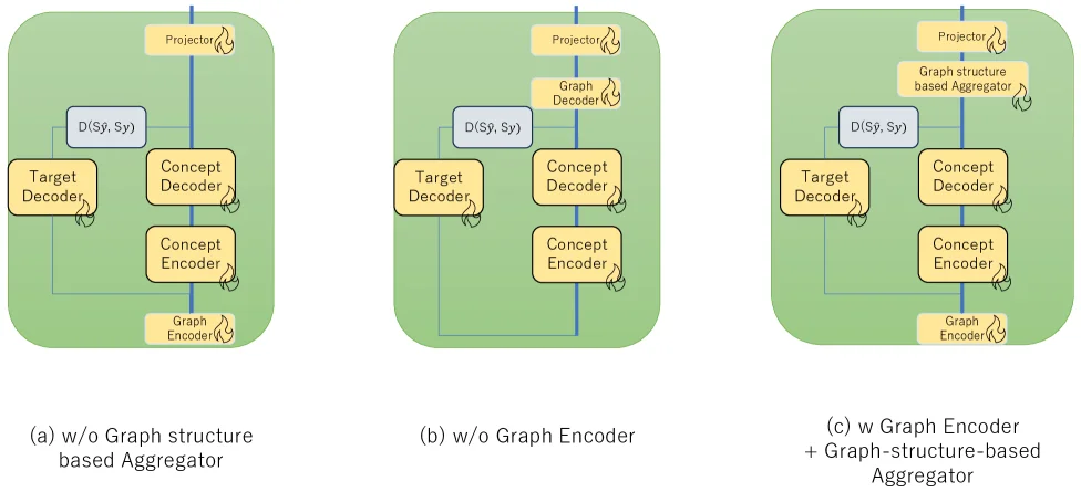
Figure H.6 : Investigation of core component arrangement: We tested our JEPA [ LeCun2022APT ] architecture with three different GNN arrangements, including (a) graph encoder only, (b) graph-structure-based aggregator only, and (c) both of them.

This figure (Figure H.6) illustrates the author's experimental investigation into three different Graph Neural Network (GNN) component arrangements for their JEPA architecture (referencing LeCun2022APT), aiming to explore how core component configurations affect model performance.

First, let's understand the meaning of each component and the direction of data flow in the diagram:

  1. Graph Encoder: Located at the bottom of each sub-figure, typically represented by a light-yellow rectangle with a flame icon (possibly indicating computation or training). Its role is to convert input graph-structured data (nodes and edges) into low-dimensional vector representations (i.e., graph embeddings). In sub-figure (a), it exists but is not subsequently connected to an aggregator; in (b), it is removed; and in (c), it exists and connects to the aggregator.

  2. Concept Encoder: Positioned above the Graph Encoder (if the Graph Encoder exists), also a light-yellow rectangle with a flame icon. It may be responsible for further processing the graph embeddings generated by the Graph Encoder or directly handling concept-related information. It is present in all three sub-figures.

  3. Concept Decoder: Located above the Concept Encoder, a light-yellow rectangle with a flame icon. Its function is to decode meaningful information from the output of the Concept Encoder, possibly for reconstruction of the input or prediction of some missing parts.

  4. Target Decoder: Located to the left of the Concept Decoder, a light-yellow rectangle with a flame icon. It may be responsible for decoding specific target information, working in conjunction with the Concept Decoder.

  5. D(Sy, Sy): A blue rectangular module connecting the Target Decoder and the Concept Decoder. It likely represents some form of distance metric or comparison function, used to evaluate the similarity or difference between the outputs of the Target Decoder and the Concept Decoder.

  6. Projector: Located at the top of each sub-figure, a light-yellow rectangle with a flame icon. Its role is to project the output from decoders or other components into a specific space for comparison or further processing.

  7. Graph-structure based Aggregator: Absent in sub-figure (a), located between the Projector and the Concept Decoder in (b), and below the Projector and above the Concept Decoder in (c). It is responsible for aggregating or processing input based on graph structural information.

Now we analyze each sub-figure (a, b, c) in detail, representing different architecture configurations and their information flow:

  • Sub-figure (a): w/o Graph structure based Aggregator (Without a Graph-Structure-Based Aggregator)

    • Data Flow: Input data is first processed by the Graph Encoder. Then, the output of the Graph Encoder is passed to the Concept Encoder. The output of the Concept Encoder is then passed to both the Concept Decoder and the Target Decoder. The outputs of the Target Decoder and Concept Decoder are fed into D(Sy, Sy) for comparison. Finally, the output of the Concept Decoder (or the result after comparison by D) is sent to the top Projector.
    • Characteristic: This configuration includes only the Graph Encoder and not a dedicated Graph-structure based Aggregator. This implies that the processing of graph structural information might be limited to the Graph Encoder stage, or handled differently in subsequent stages.
  • Sub-figure (b): w/o Graph Encoder (Without a Graph Encoder)

    • Data Flow: In this configuration, the Graph Encoder is removed. Input data directly (or with a step missing explicit graph encoding) enters the Concept Encoder. The subsequent flow is similar to (a): the output of the Concept Encoder is passed to the Concept Decoder and Target Decoder, then through D(Sy, Sy) for comparison, and finally processed by the Projector. Additionally, a Graph-structure based Aggregator is added between the Projector and the Concept Decoder.
    • Characteristic: This configuration includes only the Graph-structure based Aggregator and not the Graph Encoder. This means the model attempts to handle graph structural information using the aggregator without explicit graph encoding.
  • Sub-figure (c): w Graph Encoder + Graph-structure based Aggregator (With both Graph Encoder and Graph-Structure-Based Aggregator)

    • Data Flow: Input data is first processed by the Graph Encoder. The output of the Graph Encoder is then passed to the Concept Encoder. The output of the Concept Encoder is passed to the Concept Decoder and Target Decoder. The outputs of the Target Decoder and Concept Decoder are fed into D(Sy, Sy) for comparison. Simultaneously, the output of the Concept Decoder (or the result after comparison by D) and possibly the output of the Graph Encoder are sent to the Graph-structure based Aggregator. Finally, the output of the Graph-structure based Aggregator is sent to the top Projector.
    • Characteristic: This configuration combines both the Graph Encoder and the Graph-structure based Aggregator, aiming to fully utilize both for processing graph-structured data.

This figure reveals how the method operates by comparing the performance of the JEPA architecture under three different scenarios: 1. Using only the Graph Encoder (Figure a). 2. Using only the Graph-structure based Aggregator (Figure b). 3. Using both the Graph Encoder and the Graph-structure based Aggregator (Figure c).

Through this comparative experiment, the authors can analyze how different component combinations affect the model's understanding and processing of graph-structured data, thereby validating the importance of each component in their proposed AGE method. Although the figure does not directly show results, combining this with the paper's abstract, we can infer these experiments were conducted to optimize the model for better integration of graph-structured data as external knowledge into the generation process, addressing the misalignment issue between graph-based and text-based features in frozen LLMs. The experimental results indicate that the AGE method significantly improves the accuracy of GraphQA tasks using non-parametric search components across four benchmark datasets with distinct characteristics.

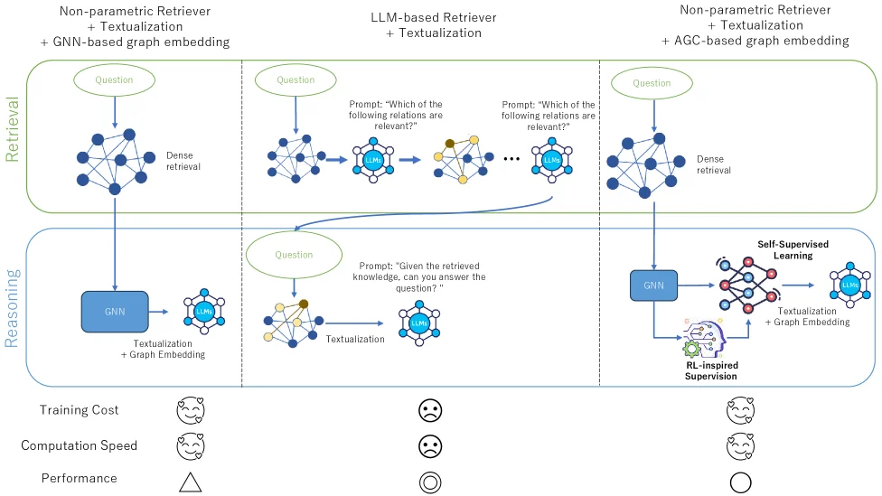
Figure H.13 : The landscape of existing KGQA methods. GNN-based methods reason on dense subgraphs as they can handle complex and graph information. LLM-based methods employ the same LLM for both retrieval and reasoning due to its ability to understand natural language.

This figure illustrates the architectures and workflows of three different Knowledge Graph Question Answering (KGQA) methods, aiming to compare their processing during the retrieval and reasoning stages, as well as their performance in terms of training cost, computation speed, and accuracy.

The figure is structured into two main parts: the upper part is the "Retrieval" stage, and the lower part is the "Reasoning" stage. There are three main columns, each representing a different method:

  1. First Column (Left): Non-parametric Retriever + Textualization + GNN-based Graph Embedding
  2. Retrieval Stage: A question is input into a dense retrieval module, which processes a graph structure (represented by blue nodes and edges). The retrieval result is passed to a GNN module for textualization and graph embedding, and then fed into an LLM for reasoning.
  3. Reasoning Stage: The GNN module processes the retrieved subgraph to extract key information, which is then passed to the LLM for final answer generation.
  4. Performance Metrics: Low training cost (smiley icon), fast computation speed (smiley icon), but moderate performance (triangle icon).

  5. Second Column (Middle): LLM-based Retriever + Textualization

  6. Retrieval Stage: A question is input into an LLM module, which retrieves relevant graph structures (represented by yellow and blue nodes) using a prompt ("Which of the following relations are relevant?"). This process may iterate multiple times (indicated by ellipsis), with the LLM refining the retrieval result in each iteration.
  7. Reasoning Stage: The retrieved graph structure is again input into the LLM with a prompt ("Given the retrieved knowledge, can you answer the question?"), and the LLM generates the final answer by combining the retrieved knowledge.
  8. Performance Metrics: High training cost (frowning icon), slow computation speed (frowning icon), but better performance (circle icon).

  9. Third Column (Right): Non-parametric Retriever + Textualization + AGC-based Graph Embedding

  10. Retrieval Stage: A question is input into a dense retrieval module, which processes the graph structure. The retrieval result is passed to a GNN module for textualization and graph embedding. Here, self-supervised learning (SSL) and reinforcement learning-inspired supervision (RL-inspired Supervision) are introduced to optimize the graph embedding process.
  11. Reasoning Stage: The GNN module processes the retrieved subgraph, combining SSL and RL-inspired supervision to extract key information, which is then fed into the LLM for final answer generation.
  12. Performance Metrics: Low training cost (smiley icon), fast computation speed (smiley icon), and best performance (circle icon).

The figure also shows the flow of data or information: - During the retrieval stage, the question is first input into the corresponding retrieval module (dense retrieval or LLM retrieval), and the retrieved graph structure is passed to the GNN module for processing. - During the reasoning stage, the information processed by the GNN module is passed to the LLM, which generates the final answer by combining the retrieved knowledge and prompts.

This figure reveals how each method works: - The first method uses a non-parametric retriever and GNN for graph embedding, suitable for handling complex graph information but with moderate performance. - The second method uses an LLM-based retriever, which can understand natural language but has high training costs and computation speed. - The third method combines a non-parametric retriever, textualization, and AGC-based graph embedding, optimizing the graph embedding process through SSL and RL-inspired supervision, achieving low training costs, high computation speed, and high performance.

Through this figure, readers can clearly see the advantages and disadvantages of each method and understand their performance differences in KGQA tasks.

← → flip · ↑ ↓ scroll notes · Esc exit